­Price Forecasting of Mango in Varanasi Market of Uttar Pradesh

Introduction

Mango being the major fruit enacts stunning role in meeting the variety of food requirements in civilized and uncivilized area of the nation. The fruit ranks first position in terms of area and that’s why it is known as king of fruits in India. Being the king of fruits, the productivity of mango crop (7.3 Mt/Ha) was much lesser than the other fruit crops (Banana-37.0 Mt/Ha, Citrus-10.3 Mt/Ha, Papaya-42.3 Mt/Ha, Guava-13.7 Mt/Ha, Apple-21.8 Mt/Ha, Grapes-15.8 Mt/Ha and Pomogranate-10.3 Mt/Ha), (Indian Horticultural Database, 2014). The yield of a crop has more effects on price of a fruit. Price of mango fruit depends upon its production and ultimately on its yield, but in some ways pre and post harvest management also affects the price of fruit. So, efforts have moreover been made to forecast price of mango on the basis of arrivals in the market and to know how it will help in reducing pre and post harvest losses of mango fruit.

Forecasts had been used traditionally in structural econometric models. At present focus were disposed on the univariate time series models known as auto regressing integrated moving average (ARIMA) models. These types of models were enormously applied for forecasting economic time series^2,6 and generalization of the exponentially weighted moving average process. A variety of techniques for recognizing special cases of ARIMA models had been suggested by Box- Jenkins¹ and others. In this paper, these models were executed to forecast the price of mango fruit in Uttar Pradesh. This would helps to predict expected price for the year 2016. Such an exercise would validate the policy makers to look forward in the future requirements for storage, import and export of mango thereby enabling them to take appropriate measures in this regard. The forecasts would thus retain much of the valuable resources of our country which otherwise would been wasted.

Methodology

Study was conducted in Uttar Pradesh as the state ranks first in the production of Mango. Out of five markets in the state, Varanasi market was selected purposively on the basis of maximum arrivals. The price data was collected from Agricultural Produce Market Committee (APMC) Varanasi for the twenty three years from 1993-94 to 2015-16. As the mango crop being seasonal in nature the data was available only for six months of the year. It was available only in the months from March to August in Uttar Pradesh. So, the data was collected only for the six months from March to August. The data was analysed with the help of E-views 7 software using the ARIMA methodology developed by Box and Jenkins.¹

In statistics Autoregressive Moving Average (ARMA) models, was also known as Box-Jenkins models after the interactive Box-Jenkins methodology usually used to estimate them and it was applied to time series data. The accuracy of forecasts for both Ex-ante and Ex-post were tested using the following tests.⁹

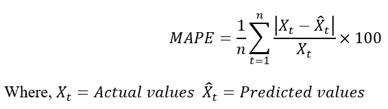
Mean average percentage error (MAPE): the formula for this is^{13,14,15,16,17}

Results and Discussion

Prices forecasting of mango in Varanasi market

The detailed results of price forecasting of mango in Varanasi market had been stated below. The above procedures were followed for forecasting the prices of mango in the Varanasi market.

Identification of the model

The Augmented Dickey-Fuller (ADF) test, Kwaitkowski-Phillips-Schmidt-Shin (KPSS) test and Phillips-Perron (PP) test were applied to test the stationarity of the data series.¹⁵ After the first difference the series found to be stationary indicating the series was integrated of order one with including the intercept only as the exogenous variable in the series.

Table 1: Stationarity test for Varanasi market price.

	ADF test		PP test		KPSS test
	Level series	1stDifferenced Series	Level series	1stDifferenced Series	Level series	1stDifferenced Series
	t-statistic	t-statistic	t-statistic	t-statistic	LM-statistic	LM-statistic
	-1.722	-7.201	-8.519	-50.068	1.246	0.409
	Critical Value for above tests
1% level	-3.483	-3.483	-3.480	-3.481	0.739	0.739
5% level	-2.884	-2.884	-2.883	-2.883	0.463	0.463
10% level	-2.579	-2.579	-2.578	-2.578	0.347	0.347

 

Figure 1: Time plot of Varanasi market price. Click here to View figure

 

From above graph it was found that there was a trend in data series. Therefore, stationarity was checked after including the trend and intercept as exogenous variable.

Table 2: Stationarity test for Varanasi market price after including Trend and Intercept as exogenous (original series)

	ADF test		PP test		KPSS test
	Level series	1stDifferenced Series	Level series	1stDifferenced Series	Level series	1stDifferenced Series
	t-statistic	t-statistic	t-statistic	t-statistic	LM-statistic	LM-statistic
	-3.116	-7.167	-10.140	-50.076	0.235	0.107
	Critical Value for above tests
1% level	-4.033	-4.033	-4.029	-4.030	0.216	0.216
5% level	-3.446	-3.446	-3.444	-3.444	0.146	0.146
10% level	-3.148	-3.148	-3.147	-3.147	0.119	0.119

 

Figure 2: Autocorrelations of original series in Varanasi market. Click here to View figure

 

Figure 3: Partial Autocorrelations of original series in Varanasi market. Click here to View figure

 

By plotting correlogram it was found that most of the coefficients of ACF and PACF were not significant. So, it was needed to seasonally differentiate the original series to get significant coefficients of ACF and PACF.¹⁰ The new seasonally differenced series was obtained from the seasonal differencing in the original price series. ADF, KPSS and PP test was used to check the stationarity in the new seasonally differenced series. The results were shown in tables 3.

Table 3: Stationarity test for Varanasi market price (Seasonally differentiated series)

	ADF test		PP test		KPSS test
	1stDifferenced Series	Level series	1stDifferenced Series	1stDifferenced Series	Level series	1stDifferenced Series
	t-statistic	t-statistic	t-statistic	t-statistic	LM-statistic	LM-statistic
	-6.868	-6.854	-8.233	-8.200	0.043	0.034
	Critical Value for above tests
1% level	-3.485	-4.036	-3.483	-4.033	0.739	0.216
5% level	-2.885	-3.447	-2.884	-3.446	0.463	0.146
10% level	-2.579	-3.148	-2.579	-3.148	0.347	0.119

 

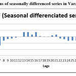Figure 4: Autocorrelations of seasonally differenced series in Varanasi market. Click here to View figure

 

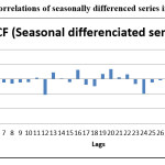Figure 5: Partial Autocorrelations of seasonally differenced series in Varanasi market. Click here to View figure

 

Estimation

It was found from the above plots of ACF and PACF (Fig 4 and Fig 5), that the values of ACF and PACF were significant¹² with seasonal differentiated series. It helps in obtaining the combinations by observing the lags of ACF and PACF, Lag of AR can be work out through PACF and lag of MA can be work out through ACF. Most probable Combinations were AR(1) MA(1), AR(1) MA(6), AR(1) MA(7), AR(6) MA(1), AR(6) MA(6) and AR(6) MA(7).

These were the most probable combinations but it had been tested for all the possible combinations up to lag observed and select the best combination for forecasting. The best combination can be selected on the basis of minimum values of Akaike Information Criteria (AIC) and Schwarz Bayesian Criteria (SBC).²¹

On the basis of minimum values of AIC and SBC it was found that AR (1) MA (6) i.e. ARIMA (1, 0, 6) model selected for the forecasting.¹⁸ Therefore, using the prices of seasonally differentiated series for the years up to 2013 and 2014, one step ahead forecast was calculate for the years of 2014 and 2015 respectively.²⁰

Diagnostic Checking

Table 4: One step ahead forecast in Varanasi market (Test for validation of the selected model)

	Actual prices (Rs/Qtl)	ARIMA forecast
		Prices (Rs/Qtl)	MAPE (%)
MAR-14	2260	2752.46	21.79
APR-14	1075	883.17	17.85
MAY-14	970	1028.32	6.01
JUN-14	860	923.87	7.43
JUL-14	865	937.89	8.43
AUG-14	1100	1096.55	0.31
MAR-15	2650	2290.39	13.57
APR-15	1380	1081.81	21.61
MAY-15	1015	1053.59	3.80
JUN-15	990	960.15	3.01
JUL-15	1040	1074.47	3.31
AUG-15	1255	1197.02	4.62

 

It was found from the above table that the model is valid by observing the Mean Absolute Percentage Error (MAPE). Average MAPE was 10.30 per cent and 8.32 per cent for the year 2014 and 2015 respectively.⁴ So, the forecasted values for the year 2016 were shown in table 11 using ARIMA (1, 0, 6) model.

Forecasting

Table 5: Out of sample forecast of Varanasi market.

	ARIMA forecast prices (Rs/Qtl)
MAR-16	2343.77
APR-16	1122.14
MAY-16	1090.04
JUN-16	995.44
JUL-16	1109.41
AUG-16	1231.87

 

Conclusion

The study concluded that the forecasted price of mango for the year 2016 was found to be highest in the start of the season. For forecasting ARIMA (1, 0, 6) model applied and revealed that there was less than 10 per cent deviation in the forecasted price of 2015 from the actual price, confirming the validity of the model. The fruit price in the start of the month was found to be almost double than the other months. It indicates that the farmers in the region has been benefited during the start of the season and to get its benefit from it they have to adopt pre and post harvest management technologies by which they can able to bring their products in market during the start of season. Our forecast results suggest fruit prices will increase during the less arrivals. These forecasts of rising prices may be encouraging signs for the farmers if they would manage their products accordingly and also it will be a guiding principle for policy makers to develop most appropriate price policy for perishable/seasonal products by which both the consumer and producer get benefitted from it.

Acknowledgements

The present paper is drawn from the PhD thesis of first author funded by BHU

References

1. Box, G. E. P. and Jenkins, G. M., Some recent advances in forecasting and control, Applied Statistics. 1968;17(2):91-109.
   CrossRef
2. Brown, R. G., Statistical Forecasting For Inventory Control. New York, McGraw-Hill, 1959.
3. Chaudhari, D. J. and Tingre, A. S., Use of ARIMA modeling for forecasting green gram prices for Maharashtra, Journal of Food Legumes. 2014;27(2):136-139.
4. Devaiah, M. C., Venkatagiriyappa and Lalith, A., Spatial integration and piece relationship of Ramanagaram over mino silk cocoon markets of Karnataka, Proceedings of the International Congress on Tropical Sericulture, Central Silk Board. 1988;77-84. [5] Gill, D. B. S. and Kumar, K., An empirical study of modeling and forecasting time series data, Indian Journal of Agricultural Economics. 2000;55(3):451-458.
5. Holt, C. C., Modigliani, F., Muth, J. F. and Simon, H. A., Planning, Production, Inventores, and Work Force. Prentice Hall, Englewood Cliffs, NJ, USA. 1960.
6. Indian Horticultural Database, National Horticulture Board, Ministry of Agriculture, Government of India, Gurgaon, 2014.
7. Iqbal, N., Bakhsh, K., Maqbool, A. and Ahmad, A. S., Use of the ARIMA model for forecasting wheat area and production in Pakistan, Journal of Agriculture & Social Sciences. 2005;1(2).
8. Makridakis, S. and Hibbon, M., Accuracy of forecasting: An empirical investigation, Journal of Royal Statistical Society. 2005;41(2):97-145:1979.
9. Naidu, G. M., Sumathi, P., Reddy, B. R. and Kumari, V. M., Forecasting price behavior of red chilli by using seasonal ARIMA model, Bioinfolet. 2014;11(1B):268-270.
10. Naik, G. and Jain, S. K., Efficiency and unbaseness of Indian commodity future markets, Indian Journal of Agricultural Economics. 2001;56(2):185-195.
11. Pal, S., Ramsubramanian, V. and Mehta S. C., Statistical models for forecasting milk production in India, Journal of Indian Society of Agricultural Statistics. 2007;61(2):80-83.
12. Paul, R. K. and Das, M. K. Statistical modelling of inland fish production in India. Journal of the Inland Fisheries Society of India. 2010;42:1-7
13. Paul, R. K. and Das, M. K., Forecasting of average annual fish landing in Ganga Basin, Fishing Chimes. 2013;33(3):51-54.
14. Paul, R. K., Forecasting wholesale price of pigeon pea using long memory time series models, Agricultural Economics Research Review. 2014;27(2):167-176.
    CrossRef
15. Paul, R. K., Panwar, S., Sarkar, S. K., Kumar, A. Singh, K. N., Farooqi, S. and Chaudhary, V. K. . Modelling and Forecasting of Meat Exports from India. Agricultural Economics Research Review. 2013;26(2):249-256
16. Paul, R. K., Alam, W. and Paul, A. K. Prospects of livestock and dairy production in India under time series framework. Indian Journal of Animal Sciences, 84(4):130-134. 2014.
17. Pradhan, P. C., Application of ARIMA model for forecasting agricultural productivity in India, Journal of Agriculture and Social Sciences. 2012;8(2):50-56.
18. Suleman, N. and Sarpong, S., Production and consumption of corn in Ghana, forecasting using ARIMA models, Asian Journal of Agricultural Sciences. 2012;4(4):249-253.
19. Wani, M. H., Paul, R. K., Bazaz, N. H. and Manzoor, M., Market integration and price forecasting of apple in India, Indian Journal of Agricultural Economics. 2015;70(2):169-181.
20. Zou, H. and Yang, Y., Combining Time Series Models for Forecasting. International Journal of Forecasting. 2004;20(1):69-84.
    CrossRef