Performance of Pulses in Gujarat: A District Level Assessment

Introduction

Pulses are versatile crops that are better for nutritional security and soil health. It is long established fact that, pulses are important part of daily diets, particularly in Asian continent. However, there has been a reduction in the consumption of pulses over the past decade. For that reason, UN declared 2016 as the international year of pulses to rekindle interest and knowledge on pulses and bring them back in to our diets.¹

India happens to be the major producer, consumer and importer of pulses;² Pulses are a chief source of protein for a massive section of Indian particularly for the poor and most of the conventionally vegetarian population.¹⁷ India accounts for 33% of the world area and 22% of the world production of pulses. Pigeon pea (Cajanuscajan), chickpea (Cicerarietinum), black gram (Vignamungo), green gram (Vignaradiata), lentils and peas are major pulses cultivated in India. About 90% of the global pigeonpea, 65% of chickpea and 37% of lentil area falls in India, corresponding to 93%, 68% and 32% of the global production, respectively.⁹

In India, pulses are grown nationwide. During the year 2014-15, total domestic production of pulses in India was 17.15 million tonnes. India imported 4.58 million tonnes of pulses and exported 0.22 million tonnes to rest of the world. During same period, total availability of pulses for domestic consumption was 21.51 million tones.³ The most important pulse producing states in India are Madhya Pradesh, Rajasthan, Maharashtra, Karnataka, Uttar Pradesh etc. Indians utilize around 30 per cent of the world’s pulses, but domestic production of pulses which become stagnated in recent time has not kept pace with population growth. The net availability of pulses has dropped from 60.70 g per day per person in 1951 to 43.30 g per day per person in 2013 as against recommendation of 65 g per day per person by Indian council of Medical Research.⁴ Import of pulses in India has increased, it currently accounts for about 15–20 per cent of total domestic availability. Canada, Myanmar, Australia and Tanzania are the foremost exporters of pulses to India.

The growth of pulses has always been unenthusiastic in spite of the remarkable growth of Indian agriculture. The Ministry of Agriculture and Cooperation has focused on improving pulse production through various programme like Technology Mission (1986), National Pulse Development Project (1990-91), Integrated scheme of Oilseeds, Pulses, Oil palm and Maize (2004), National Food Security Mission (2007-08) and A3P i.e. Accelerated Pulses Production Programme but supply always stay behind the demand and country has to greatly relied on imports to meet up the supply-demand gap.

Performance of Pulses in major states have become stagnated and minor pulse producing states have real potential in pulse development programme as yield of pulse crops in these minor states was higher than the national average.²⁵ These states might bring real breakthrough in pulse production in India by which we can reduce import dependency, stabilize the prices of pulses, reduce food inflation and save valuable foreign currency. Gujarat is recognized as one of the minor pulse producing states.²⁵ This state is having potential to contribute in pulse production at national level. In recent times, the state has achieved spectacular growth in agriculture sector including pulses among all Indian states.¹¹ Hence his research was undertaken to study the performance of pulses at state and district level. Similarly, study also aims to identify the major districts, which have recorded sustainable growth with stability in its yield.

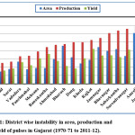Figure 1: District wise instability in area, production and yield of pulses in Gujarat (1970-71 to 2011-12). Click here to View figure

 

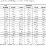Table 1: Growth rates of area, production and yield of pulses in various districts of Gujarat. Click here to View table

 

Materials and Methods

The Study Area

This particular study was undertaken in Gujarat. Major Eighteen agricultural districts of Gujarat state namely Ahmedabad, Amreli, Banaskantha, Bharuch, Baroda (Vadodara), Bhavnagar, Valsad, Dang, Jamnagar, Junagadh, Kheda, Kutch, Mehsana, Panchmahal, Rajkot, Sabarkantha, Surat and Surendranagar (As per 1971 census) were covered under present study.

Data

Districts are the lowest administrative unit at which reliable agricultural data is available in Gujarat hence performance of cotton was analysed  at district level along with state. Secondary time seies data of area, production and yield (APY) were collected from various sources. viz; Season and Crop Reports, Department of Economics and Statistics (DES), Government of Gujarat, online data bank of International Crop Research Institute for Semi-Arid Tropics²⁶ and Economic and Political Weekly (EPW) data bank [www.epwrfits.in]. The data were collected for the years from 1970-71 to 2011-12. The CGR and instability were estimated for overall period i.e. 1971-72 to 2011-12 and two sub-periods. These sub-periods approximately represents phase of green revolution and post-green revolution. The period-I starts from the year 1971-72 to 1989-90, which represent a period of green revaluation. Second period (Period-II) starts from the year 1991-92 to 2011-12. This period was known as post green revolution period in which we have seen wider dissemination of technology.⁵

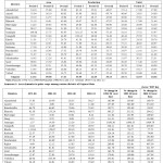Table 2: Instability in area, production and yield of pulses in various districts of Gujarat Click here to View table

 

Analytical Tools

Growth

The growth rateswere estimated based on its fit using non linear models, especially, the exponential model. The exponential model is more commonly used in econometric analysis. Usually, the compound growth rates were estimated after converting the growth model to semi-log form and estimated through Ordinary Least Square (OLS) technique assuming multiplicative error term.

Y_t = b₀ * b₁^t * e_t———————————[1]

ln (Y_t) = b₀+t * ln b₁ +e_t —————————[2]

Where,

ln (Y_t) is the natural logarithm of time series data for area / production / yield for year t,

b₀ is the constant term,

t is the time trends for years of interest,

e_t is the error term and

b₁ is growth rate for the period under consideration (i.e. slope coefficient).

Then, Compound growth rate was calculated using following equation

Compound Growth Rate = [(Antilog b₁)-1]*100  ————-[3]

But, this method have  several problems including the difficulty in estimating standard error of estimates of original parameters.¹⁸ Thus, a non-linear estimation technique for solving exponential model assuming additive error terms were employed to estimate the compound growth rates.

Y_t = constant *(1+CGR)^t +e_t  ————————————-[4]

Where,

Y_t is the time series data for area / production / yield for year t,

t is the time trends for years of interest,

e_tis the error term and

CGR is compound growth rate for the period under consideration

The data were smoothened with the help of three year central moving average techniques to remove bias from the data if any induced by the outliers [Sawant, 1983; Sawant and Achuthan, 2007 and Singh et al., 1997]. The Marquardt algorithm was used to estimate the parameters of equation.⁴ The significance of regression coefficient ‘b’ (slope coefficient) was tested by applying standard ‘t’ test procedure [Gujarati and Sangeetha, 2007].

Instability

The method that may use to examine instability in a variable over time should satisfy two minimum conditions. First, it should not include deviations in the data series that arise due to secular trend or growth. Second, it should be comparable across the data sets having different means [Mehra, 1981 and Hazell, 1984]. Simple coefficient of variation (CV) overestimates the level of instability in time series data, characterised by the long-term trends. To avoide the problem of overestimation, Cuddy-Della Valle, 1978 ; Mehra, 1981 ; Hazell, 1982 ; and Ray, 1983  have propsed alternative methods to estimate instability in time series data.  However, Mehra, 1981  and Hazell, 1982 methods have been criticized  for measuring instability around arbitrarily assumed trend line, which greatly influences inference regarding changes in instability, hence these two methods were not slected in present study. In recent time, international fraternity have mostly used Cuddy-Della Valle Index to measure the instability because of its supearity over other methods [Weber and Sievers, 1985; Singh and Byerlee, 1990 and Deb et al., 2004], hence we have used Cuddy-Della Valle Index as a measure of variability in the present study. This index is a modification of coefficient of variation [CV] to accommodate trend, which is commonly present in time series economic data. It is superior over other scale dependent measures such as Standard Deviation or Root Mean Square of the residuals (RMSE) obtained from the fitted trend lines of the raw data, and hence suitable for cross comparisons [Cuddy and Della Valla, 1978 and Della Valle, 1979].

The Cuddy-Della Valle Index (I_x) was calculated as follows:

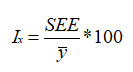
Where,

Ix = Instability index

SEE  =  Standard error of the trend line estimates

Y^–= Average value of the time series data

The SAS macros for econometric analysis-I  available on web adrees of Indian Agricultural Statistical Research Institute, New Delhi (http :// www. iasri. res. In / sscnars / ecoanlysis.aspx) was used to analyse the data with the help of Statistical Analysis System (SAS) software, Version 9.3.[www.iasri.res.in].

Results and Discussion

Growth

The annual compound growth rate (CGR) in area of pulse crops was 3.91, -0.84 and 0.76 per cent per annum during two sub-periods and overall period at state level, respectively (Table 1). It was statistically significant at 1 per cent level of significance. This shows that, maximum growth in area of pulse crops has been occurred during first period (1971-1990). During second period, area under pulse crops was decreased. Yield of pulse crops has shown positive and significant trend in all the three period of study but maximum growth was observed during first period. The CGR of yield during two sub-periods and overall period was 2.57, 1.71 and 1.44 per cent, respectively. The positive growth in area and yield during first period leads significant high positive growth in production of pulse crops i.e. 5.48 per cent per annum.  Positive and significant trend in production of pulse crops was also seen in overall period. During this period CGR of production was medium (1.77 per cent per annum).

The district level results shows that, in first sub-period of study (1971-1990), except Valsad district all the districts has shown positive trend in area of pulse crops but high CGR i.e. more than 3 per cent was recorded in Ahmedabad, Bharuch, Jamnagar, Junagadh, Rajkot, Sabarkantha, Surendranagar and Vadodara districts. During second sub-period, many of the districts shown negative trends in area of pulse crops.  Important of them were Banaskantha, Bharuch, Kheda, Sabarkantha, Surat, Surendranagar and Vadodara districts. Only few districts viz; Amreli, Jamnagar, Junagadh, Mehsana and Rajkot districts have shown positive trend in area of pulse crops in second sub-period of study. In overall period, except Kachchh, Valsad and Kheda, rest of the districts have registered positive trend in area of pulse crops.

Magnitude of CGR in regards to production and yield of pulses was seen higher in first sub-period compared to second sub-period of study. Few districts viz; Amreli, Junagadh, Kachchh and Surendranagar have registered prominent CGR in yield and production during second sub-period. In overall period, all the districts have shown positive trend in production and yield of pulse crops. (Except production of pulse crops in Valsad district)

Only one district i.e. Jamnagar has registered high (More than 3 per cent) CGR in yield of pulse crops in overall period. Rest of the districts has seen low to medium (Between 0 to 3 per cent) level of CGR in yield of pulse crops. During overall period, production of pulse crops was seen high in Amreli, Jamnagar, Junagadh, Panchmahal, Rajkot and Surendranagar districts where magnitude of CGR was greater than 3 per cent per annum. During first sub period, area expansion coupled with yield improvement was a reason for increase in production of pulse crops in the state but during second period, increase in production was mainly comes from improvement in the yield of pulse crops. Results of decomposition analysis reported by More et al., 2015   also stated that, improvement in yield of pulse crops was the main reason behind the increase in production followed by interaction of yield in to area which supports our view.

Instability

State and district level estimates of instability in regards to area, production and yield of pulse crops for three periods viz; 1971-1990, 1991-2012 and 1971-2012 were presented in table 2 and figure 1.

In Gujarat state, instability in area of pulse crops during the study periods was 13.42, 9.08 and 17.31 per cent per annum, respectively. Area under pulse crops in the state was relatively stable in second sub-period compared to first. Similarly, production and yield of pulse crops was also stable in second sub-period compared to first sub-period. Instability in production of pulse crops was reduced to 22.65 per cent from 35.90 per cent in sub-sequent periods. Instability in yield was also decreased to 16.93 per cent from 25.72 per cent. Yield variability in pulse crops was relatively higher than area variations which again clearly indicated that, yield variation was a major source of variation in production of pulsecrops in the state. A study by Mehta (2013) alsomentioned similar resultson the yield of pulse crops being mostly unstable compared to area in the Gujarat state.

District level results shows that, during first sub-period, instability in area of pulse crops was ranged from 6.66 per cent (Valsad) to 104.66 per cent (Jamnagar) and during second sub-period, it was ranged from 6.69 per cent (Vadodara) to 56.10 per cent (Amreli). During first sub-period of study, low level of instability was seen in Valsad, Dang and Surat districts and high level of instability was recorded in Jamnagar, Junagadh, Amreli, Rajkot, Kachchh and Ahmedabad districts. In rest of the districts, instability in area of pulse crop was moderate.

In second sub-period of study, many of the districts except Amreli, Panchmahal, Surat, Kheda, Surendranagar, Valsad, Dang and Bhavnagar showed decrease in the level of area instability in pulse crops which is good sign. Among these districts, maximum increase of instability was seen in Dang and Bhavnagar districts.

It is obvious that, magnitude of production instability of pulse crops was high compared to its area and yield. Such type of results is seen because production is interaction of area and yield series.  The range of instability in production of pulse crops was from 24.46 per cent (Valsad) to 108.16 per cent (Junagadh) in first sub-period and from 15.64 per cent (Surat) to 64.80 per cent (Bhavnagar) in second sub-period of the study. In both the periods, moderate to high level of production instability was seen in various districts of Gujarat state.

When compared to first sub-period, instability in production of pulse crops was reduced in second sub-period except in Panchmahal, Bhavnagar, Surendranagar and Dang districts.

Lowest level of yield instability in pulse crops was recorded in Surat (20.26 per cent) and Valsad (10.60 per cent) districts during first and second sub-period of the study, respectively whereas highest level of yield instability was seen in Kachchh (57.21 and 40.65 per cent)  district during both the sub-period of the study.Even though the magnitude of yield instability was reduced in second sub-period of study, moderate to high level of instability in yield of pulse crops was observed in various districts of Gujarat state.  Instability in yield was reduced utmost in Amreli followed by Junagadh, Mehsana, Ahmedabad, Vadodara, Bhavnagar, Kachchh etc. districts. In Panchmahal, Surat, Sabarkantha and Banaskantha districts, instability in yield were reduced marginally i.e. less than 5 per cent.

Conclusion

The production of pulse crops was recorded to increase in Gujarat during entire study period. The increase in pulse crops in the state was due to area expansion coupled with marginal improvement in yield up to the year 1990 after that, increase in production was mainly from improvement in the yield of pulse crops as area was stagnated. Area under pulse crop was increased consistently up to year 1990 afterwards it was stagnated. Consistent improvement in the yield of pulses was a notable feature which shows that improved technology has payoff in the state. High growth in area, production and yield of pulse crops was associated with high level of instability during first sub period.Yield variability in pulse crops was relatively higher than area variations which clearly indicated that yield instability was a major source of variation in the production of pulse crops. Hence efforts should be made to stabilize the yield level in pulse crops.

Reference

1. Anonymous. Farmers and consumers need to be pulse smart. www.icrisat.org/famers-and-consumers-need-to-be-pulse-smart. 2016a
2. Anonymous.  Agriculture: More from less. Economic Survey 2015-16, Ministry of Finance, Government of India. 2016b;70
3. Anonymous.  Commodity profile for pulses-March, 2016. www.agricoop.nic.in/imagedefault/trade/pulses.pdf. 2016c
4. Anonymous.   Economic survey 2015-16 technical appendix. Economic Survey2015-16, Ministry of Finance, Government of India. 20016d;A36.
5. Chand, R., and Raju, S. S.  Instability in Indian agriculture. National Centre for Agricultural Economics and Policy Research. New Delhi: National Centre for Agricultural Economics and Policy Research. 2008.
6. Cuddy, J. A., and Della Valla, P. A. Measuring the instability in time series data. Oxford Bulletin of Economics and Statistics. 1978;40(1):79-85.
   CrossRef
7. Deb, U. K., Bantilan, M., Evenson, R. E., and Roy, A. D.  Productivity impact of improved sorghum cultivars. In : Bantilan, M., Deb, U.K., Gowda, C., Reddy, B., Obilana, B.A.D., and Evenson, R.E. Sorghum genetic enhancement : research. process, dissemination and impacts. Patancheru, Andhra Pradesh, India: ICRISAT. 2004;203-222.
8. Della Valle, P.A.  On the instability index of time series data : A generalization. Oxford Bulletin of Economics and Statistics. 1979;41(3):247-248.
   CrossRef
9. FAO STAT (2012). FAO-Statistical Database.(www.faostat.fao.org.)
10. Gujarati, D. N., and Sangeetha. Basic econometrics. New Delhi: Tata McGraw Hill Education, Pvt. Limited. 2007
11. Gulati, A., Shah, T., and Ganga, S. Agriculture performance in Gujarat since 2000: Can it be a Divadandi for other States? New Delhi: International Food Policy Research Institute. 2009.
12. Hazell, P. B. Instability in Indian Foodgrain Production. Washington, D.C.,USA: International Food Policy Research Institute. 1982.
13. Hazell, P.B. Sources of increased instability in Indian and U.S. cereal production. Washington DC: International Food Policy Research Institute. 1984.
14. http://www.epwrfits.in/. (n.d). Retrieved October 12, 2014 from http://www. epwrfits.in/ICSSRAdvt.aspx.
15. Mehra, S.  Instability in Indian agriculture in the context of the new technology. Washington DC., USA: International Food Policy Research Institute. 1981.
16. Mehta, N. Performance of Crop Sector in Gujarat during High Growth Period: Some Explorations. Agricultural Economics Research Review. 2012;25(2):195-204.
17. Reddy, A.A. Consumption pattern, trade and production potential of pulses. Economic and Political Weekly. 2004;39(44):4854-4860.
    CrossRef
18. Prajneshu, and Chandran, K.P. Computation of compound growth rate in agriculture: Revisited. Agricultural Economics Research Review. 2005;18:317-324.
19. Ray, S.K. An empirical investigation of the nature and causes for growth and instability in India : 1950-80. Indian Journal of Agricultural Economics. 1983;38(4):459-474.
20. SAS Macro (n.d.) The SAS macros for econometric analysis-I Retrieved January 22, 2014, from http:// www.iasri.res.in /sscnars / ecoanlysis .aspx.
21. Sawant, S.D. Investigation of the hypothesis of deceleration in Indian agriculture. Indian Journal of Agricultural Economics. 1983;38(4):475-496.
22. Sawant, S.D., and Achuthan, C.V. Agricultural growth across crops and regions: Emerging trends and patterns. Economic and Political Weekly. 1995;30(12):2-13
23. Singh, A.J., and Byerlee, D. Relative variability in wheat yields across countries and overtime. Journal of Agricultural Economics. 1990;41(1):21-32:.
    CrossRef
24. Singh, I.J., Rai, K.N., and Karwasra, J.C.  Regional variations in agricultural performance in India. Indian Journal of Agricultural Research. 1997;52(3):374-386.
25. Srivastava, S. K., Sivaramane, N., and Mathur, V. C.  Diagnosis of Pulses Performance of India. Agricultural Economics Research Review. 2010;23(1):137-148.
26. VDSA. Village dynamics in south Asia (VDSA) database, generated by ICRISAT/IRRI/NCAP in partnership with national institutes in India and Bangladesh. 2013. (http://vdsa.icrisat.ac.in).
27. Weber, A., and Sievers, M.  Observations on the geopraphy of wheat production instability. Quarterly Journal of International Agriculture. 24(3):1985;201-211.