Determining the Impact of Rainfall on Major Crop Yields in Tamil Nadu using Vector Error Correction Model

Introduction

Agricultural crops play a vital role in shaping the economy, culture, and livelihoods of Tamil Nadu. As one of India’s foremost agricultural states, Tamil Nadu benefits from a diverse range of agro-climatic zones, enabling the cultivation of an extensive array of crops such as rice, sugarcane, cotton, millets, groundnuts, and horticultural produce including bananas and mangoes. The agricultural sector not only provides employment to a large segment of the rural population but also contributes notably to the state’s Gross Domestic Product (GDP). Staple crops like rice are central to ensuring food security, while cash crops such as sugarcane and cotton fuel key industrial sectors, including sugar refining and textile manufacturing. Furthermore, the state’s rich horticultural output enhances its export prospects and supports broader goals of nutritional security. The sector also supports allied activities like dairy, fisheries, and poultry, creating a synergistic effect on rural development. With sustainable practices and technology adoption, agriculture remains a cornerstone of Tamil Nadu’s socio-economic progress. In recent years, the focus on agricultural development in Tamil Nadu has extended to modernizing farming practices, adopting water-efficient techniques, and promoting climate-resilient crops. These efforts aim to address the challenges of changing climatic conditions and ensure sustainable agricultural growth in the state.

Time series analysis plays a critical role in agricultural forecasting by facilitating data-driven predictions and informed decision-making. Agriculture is inherently influenced by seasonal patterns, climatic variations, and market trends, all of which can be effectively analyzed using time series techniques. By examining historical data, time series models help forecast crop yields, rainfall patterns, pest outbreaks, and market prices, providing valuable insights for farmers, policymakers, and agribusinesses. Accurate forecasts enable better planning for sowing, irrigation, harvesting, and marketing, minimizing risks and maximizing productivity. Time series methods such as Autoregressive Integrated Moving Average (ARIMA), Seasonal Autoregressive Integrated Moving Average (SARIMA), Vector Autoregressive (VAR) models, VECM, and exponential smoothing capture trends, seasonality, and cyclic behavior, offering reliable predictions. In a rapidly changing agricultural landscape, these tools contribute to sustainable farming practices, food security, and economic stability.

Multivariate time series analysis involves examining and modeling the relationships among multiple time-dependent variables to understand their interactions and predict future behavior. Unlike univariate analysis, which focuses on a single variable, multivariate techniques account for the dynamic interplay among variables, capturing their mutual influence over time. This approach is widely used in fields such as economics, agriculture, and environmental science, where interdependent variables often influence outcomes. Methods like VAR, VECM, and Cointegration Analysis are commonly applied in multivariate time series analysis to identify long-term equilibrium relationships, study causality, and forecast complex systems. This comprehensive approach enables deeper insights and more accurate predictions in dynamic, interconnected systems.

The VECM is highly significant in agriculture, particularly in analyzing and forecasting interdependent economic and environmental variables. Agriculture is influenced by multiple interconnected factors such as rainfall, crop prices, input costs, and global market trends. VECM is specifically designed to handle non-stationary time-series data that exhibit long-term equilibrium relationships, making it a powerful tool for agricultural studies. By identifying cointegration among variables, VECM captures both short-term dynamics and long-term equilibrium, enabling more accurate predictions and policy analysis. For example, it helps in understanding how changes in one variable, such as fertilizer prices, can impact crop yields or market prices over time. This insight is crucial for developing strategies to stabilize agricultural markets, optimize resource allocation, and ensure food security.

Jabarali et al.,¹ successfully demonstrates the effectiveness of the Vector Error Correction (VEC) model in forecasting carbon dioxide emissions in India. By incorporating a dynamic specification, the model reveals that GDP, energy consumption, and trade have a long-run equilibrium relationship with carbon dioxide emissions, as validated through Johansen’s cointegration analysis. The VEC model’s forecasting accuracy surpasses that of ARIMA and VAR models, highlighting its reliability in predicting emissions based on economic indicators. This advanced multivariate approach provides a robust framework for understanding the interplay between economic activities and environmental impacts, making it a valuable tool for policy planning and emission control strategies.

Literature Reviews

A literature review provides a crucial foundation for research, offering insights into existing knowledge, theories, and findings relevant to the topic. The following review is highly beneficial for this study.           Salmon² provides a foundational exploration of error correction mechanisms, offering significant advancements in both their theoretical and practical applications. By critically addressing the limitations of ad hoc dynamic specifications, the paper introduces robust modeling approaches, such as the Proportional-Integral-Derivative rule, to bridge short-run dynamics with long-term equilibrium behavior. This work establishes a robust framework for resilient and sophisticated econometric modeling, paving the way for improved decision-making under uncertainty. Nonetheless, the inclusion of empirical validation and practical case studies would further bolster its applicability and enhance its relevance across diverse economic scenarios.

The seminal work by Engle and Granger,³ along with its extensions, offers a foundational framework for understanding cointegration and error correction models. Its theoretical rigor, combined with practical methodologies and empirical examples, makes it an indispensable reference in the study of time series econometrics. However, further advancements could focus on improving computational efficiency and enhancing applicability in multivariate and small-sample scenarios.

Awosola et al.,⁴ used Johansen’s cointegration approach to analyze the impact of price, non-price factors, and natural disincentives on agricultural growth in Nigeria. Using time-series data from the Central Bank of Nigeria, they found a long-run price elasticity of supply of 0.13 and an 18% supply shift attributed to capital, highlighting the need for further research to address factors affecting supply responses and enhance agricultural sustainability. Wong and Ng⁵ developed an econometric model for forecasting the Tender Price Index (TPI) in construction, using Johansen’s multivariate cointegration analysis. Their model shows TPI is cointegrated with GDP, construction output, and building costs, and employs a Vector Error Correction (VEC) model to predict TPI movements achieving a low mean absolute percentage error of 2.9% over three years. The VEC model outperforms traditional methods like Box-Jenkins and regression models, offering reliable short- to medium-term forecasts. While focused on Hong Kong, the approach can be applied to other economic variables, enhancing forecasting accuracy and supporting public sector planning.

Andrei, D. M. and Andrei, L. C,⁶ investigates the long- and short-run relationships among key macroeconomic variables in Romania—foreign direct investment, imports, exports, GDP, and labor—while considering the influence of the 2008–2012 economic crisis. Using the Johansen cointegration test and a VECM, the study identifies significant cointegration among the variables, revealing that foreign direct investments strongly impacts other macroeconomic indicators both positively and negatively. The Granger causality test highlights directional relationships, showing the crisis significantly affected foreign direct investments, imports, exports, and GDP, but not labor.

Usman et al.,⁷ effectively demonstrates the utility of VECM in modeling the interactions between PIR, PIP, and FTT, offering valuable insights into the dynamics of farmers’ terms of trade in Indonesia. The findings highlight the dominant role of prices received by farmers in shaping trade terms, with shocks in PIP having a relatively smaller impact. While the study is methodologically robust, its impact could be enhanced with a broader temporal scope and exploration of external influences. Nonetheless, it makes a significant contribution to agricultural economics and offers practical insights for policymakers.

Asari et al.,⁸ analyze the dynamic relationships between interest rates, inflation, and exchange rate volatility in Malaysia (1999-2009) using a VECM framework. Their findings reveal that inflation causes interest rate changes, which in turn affect exchange rate volatility. Interest rates positively impact exchange rates in the long term, while inflation has a negative effect. The study suggests raising interest rates to mitigate exchange rate volatility and calls for further research with panel data and additional variables to refine these relationships.

Senthamaraikannan et al.,⁹ conducted a study aimed at exploring the interrelationships among agricultural commodities using a co-integration test. Their analysis revealed a significant long-term relationship among the endogenous variables. By employing the VECM, the study estimated key parameters, which were subsequently used to forecast rice production for the years 2017 and 2018. The findings offer valuable insights to enhance agricultural planning and inform data-driven decision-making in the agricultural sector. Montaño et al.,¹⁰ examined the relationship between agriculture and energy prices over four decades. The study found that changes in agricultural prices influenced energy prices due to supply-demand imbalances driven by high-protein diets, rising biofuel demand, and global trade distortions. Additionally, climate-induced droughts and floods increased energy demand in agriculture to mitigate climate impacts. The findings highlight the interconnected roles of energy as both an input and output in the agricultural sector.

Amassaib et al.,¹¹ employed the co-integration VEC model to examine market efficiency in Elobied Crops Market for sesame, groundnut, and Arabic gum. The random walk test and VEC models revealed a weak form of EMH for sesame and groundnut but semi-strong EMH for Arabic gum. The study highlighted that small changes in demand significantly impact prices due to price flexibilities, emphasizing the need for improved information accessibility to enhance market efficiency and mitigate risks from inadequate market information.

Matulessy¹² utilized the VECM approach to analyze rainfall dynamics, highlighting that long-term rainfall changes are influenced by previous rainfall and irradiation, while short-term fluctuations are influenced solely by previous irradiation levels. The study showed that VECM outperforms the ARIMA(1,0,2) model in forecasting rainfall.

Kamalanathan et al.,¹³ applied Markov chain models to forecast daily fruit price movements in Salem District, Tamil Nadu. By categorizing price changes into gain, loss, and no change, they develop models to analyze transitions for ten fruits, calculating metrics like transitional and steady-state probabilities. The results suggest a higher likelihood of price gains than losses, highlighting the potential of Markov chains in predicting agricultural price trends and supporting investment in the fruit market. Drawing from the valuable insights provided in the above review, this study is conducted to delve deeper into the subject and address the gaps identified, with the aim of advancing understanding and providing solutions using Python programming.

Materials and Methods

Study Area and Data Description

The study focuses on Tamil Nadu, a state in southern India with a predominantly agrarian economy, where rainfall significantly impacts agricultural production. Annual data on major crop yields (e.g., Cholam, Cumbu, and Maize) and rainfall for the time period 1990-91 to 2022-23 were collected from the official website of the Department of Economics and Statistics, Government of Tamil Nadu, India (https://www.tn.gov.in/crop/stat.html).

Table 1: Basic Statistics

BasicStatistics	Rainfall(in mm)	Cholam(in Tonnes)	Cumbu(in Tonnes)	Maize(in Tonnes)
Maximum	1401.1	868940	296270	2989945
Minimum	598.1	153856	56505	43820
Mean	973.47	363440.03	155494.72	1043979.06
Median	985.8	345820	146132	759112
Skewness	0.1087	1.25	0.48	0.69
Kurtosis	-0.6067	2.75	-0.65	-1.20
SD	190.4448	145036.983	61790.6097	1070031.06

Table 1, provides an overview of the key statistical characteristics of the dataset utilized in this study. The VECM was employed to analyze the long-term and short-term relationships between rainfall and crop yields. Below is a detailed explanation of the methodological approach.

Kwiatkowski-Phillips-Schmidt-Shin (KPSS) Test

VECM is used when the variables are non-stationary but cointegrated. Hence, identifying whether a series is stationary or not is crucial. The KPSS test is a statistical method used to assess the stationarity of a time series, determining whether it has a constant mean and variance over time. Specifically, it tests the null hypothesis that a time series is stationary around a constant or a deterministic trend (depending on the type of test), against the alternative hypothesis that the series is non-stationary. This test statistic is based on the residual sum of squares (RSS) from a regression model of the time series. The formula for the KPSS statistic is:

wehre T is the length of the time series (number of observations), û are the residuals from the regression (i.e., the difference between the actual values and the estimated trend or constant) and σ² is the estimated variance of the residuals.

Johansen Cointegration Test

Johansen¹⁴ presents a statistical framework for analyzing nonstationary Vector Autoregressive (VAR) processes integrated of order 1, emphasizing their cointegration properties. Kamalanathan et al.,¹⁵ conducted a comprehensive analysis of agricultural product dynamics by employing the Granger Causality Test to examine the directional relationships between variables, Impulse Response Functions to assess the impact of shocks over time, and the Augmented Dickey-Fuller (ADF) Test to evaluate the stationarity of the data. These econometric techniques provided valuable insights into the interdependencies and long-term behavior of agricultural markets. The study introduces a maximum likelihood estimator for identifying the cointegration space and proposes a likelihood ratio test to determine the number of cointegration vectors. Furthermore, it outlines methods for testing linear hypotheses about the cointegration vectors. This test is particularly crucial for the VECM, as the VECM requires that the variables are cointegrated to establish meaningful long-term equilibrium relationships. By identifying cointegration, the Johansen test provides the foundation for specifying the VECM, allowing the model to capture both short-term dynamics and long-term relationships between the variables. The Johansen test is derived from a Vector Autoregressive (VAR) model of order 𝑝:

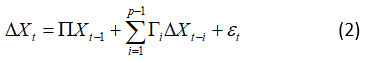
where X_t is a vector of k-dimensional time series variables, ΔX_t is the first-difference operator, Γ_i is short-run coefficient matrices ∏ is a Long-run impact matrix, and ε_t is the error term.

Variance Decomposition

The Johansen test focuses on the decomposition of the long-run impact matrix ∏, which is a key component in identifying cointegrating relationships among variables. The matrix ∏ is expressed as the product of two matrices,

where β represents the matrix of cointegrating vectors of order k×r that capture the long-term equilibrium relationships between the variables, and α the matrix of order k×r  adjustment coefficients, which measure the speed at which the system corrects deviations from the equilibrium. This decomposition allows the Johansen test to determine both the number and the structure of cointegrating relationships in the system.

Vector Error Correction Model

For k variables with p lags, the VECM equation is

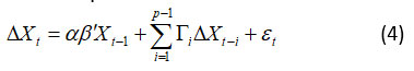
where ΔX_t is changes in the variables(short run dynamics), αβ’X_{t -1} is cointegrating relationship (long-term equilibrium), α is adjustment coefficients (speed of returning to equilibrium), Γ_i Short-run coefficients capturing lagged effects of differences, and ε_t is the error term.

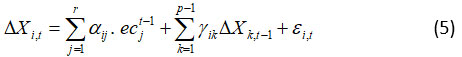
where ec_j^{t -1} =β’_j X_{t -1} is the cointegration equation. In the context of a VECM, the equation for each variable X_i,t can be expressed in its expanded form. This formulation illustrates how the changes in a particular variable are influenced by the lagged differences of all variables in the system, as well as by the error correction term. The error correction term reflects the extent to which the system deviates from the long-run equilibrium, with adjustments occurring over time to restore the balance. This expanded representation provides a detailed view of the dynamic interrelationships and long-run dependencies among the variables in the system.

Impulse Response Functions

An Impulse Response Function (IRF) quantifies the dynamic response of a system’s variables to a one-time, unitary shock (impulse) in one specific variable, while holding all other shocks constant at zero. Widely utilized in time-series modeling frameworks such as VAR and VECM, the IRF traces the propagation of this shock throughout the system over time. By capturing the temporal interactions and feedback mechanisms among variables, it provides critical insights into the short-term and long-term dynamics of the system, enabling researchers to assess the extent, direction, and persistence of the effects triggered by the initial disturbance.

IRF is derived by transforming the VAR model into a more interpretable format using the lag operator. In a VAR(p) model, which represents the relationship between variables in a multivariate time series, the dynamic structure is captured by incorporating lagged values of the variables. By applying the lag operator, the model is reformulated into its moving average (MA) representation, enabling us to express the current and future values of the variables as a function of past innovations (shocks). This transformation lays the foundation for calculating the IRF, as it isolates the effects of a one-time unit shock in a specific variable, while keeping all other shocks constant, and traces its influence on all variables over time. This approach provides critical insights into the dynamic interdependencies and causal relationships within the system.

where Φ(L) represents the moving average representation of the VAR model. The response of Y_t+h to a shock at time 𝑡 is given by:

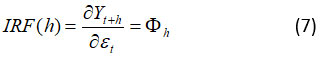
where Φ_h​ is the coefficient matrix at horizon h in the moving average representation.

Outcome Analysis and Discussion

KPSS Test

Table 2, highlights the KPSS test results for the Cholam, Cumbu, and Maize series, indicating their stationarity properties:

Cholam: The KPSS statistic (0.5940) exceeds the critical values at all significance levels, and the p-value (0.015) is below the 0.05 significance threshold.

Cumbu: The KPSS statistic (0.5887) also surpasses all critical values, with a p-value (0.0237) less than 0.05.

Maize: Similarly, the KPSS statistic (0.8624) is higher than all critical values, and the p-value (0.01) is below the 0.05 significance level.

Table 2: Result of KPSS Test

Crops	Test Statistic	P – value
Cholam	0.5940	0.015
Cumbu	0.5887	0.023
Maize	0.8624	0,010
*Critical Values (10%: 0.347), (5%: 0.463), (2.5%: 0.574), (1%: 0.739)

For all three crops, we reject the null hypothesis of stationarity. This implies that the time series for Cholam, Cumbu, and Maize are likely non-stationary, exhibiting trends, seasonality, or fluctuating variance over time. To ensure these series are suitable for time-series modeling, transformations such as differencing are recommended to achieve stationarity.

Table 3: Selection of Optimal Lag Order

Lag Order	AIC	BIC	HQIC
0	81.95	83.12	82.06
1	81.16	83.12	81.35
2	76.13	78.87	76.40
3	-64.50	-60.97	-64.15
4	-144.6	-140.3	-144.2
5	-166.0	-160.9	-165.5
6	-164.9	-159.0	-164.3
7	-167.7*	-161.0*	-167.0*

Table 3, presents the results of selecting the optimal lag order for a time series model based on three criteria: AIC (Akaike Information Criterion), BIC (Bayesian Information Criterion), and HQIC (Hannan-Quinn Information Criterion). Each criterion evaluates model fit by balancing goodness-of-fit with model complexity, where lower values indicate better model performance. The lowest values for all three criteria (AIC, BIC, HQIC) are marked with an asterisk (*) at lag order 7, indicating it is the best choice.

Result of Johansen Cointegration Test

From the table 4, it is observe that

Cholam

The trace test indicates, for r=0, the trace statistic (15.777) exceeds the critical value (15.494) at the 5% significance level, so we reject the null hypothesis of no cointegration and conclude that at least one cointegrating relationship exists and for 𝑟≤1, the trace statistic (5.498) is greater than the critical value (3.841), so we reject the null hypothesis of at most one cointegrating relationship. The max eigenvalue test, for 𝑟=0, The max eigenvalue statistic (10.279) is less than the critical value (14.263), so we fail to reject the null hypothesis of no cointegration and for r=1, the max eigenvalue statistic (5.498) exceeds the critical value (3.841), so we reject the null hypothesis of at most one cointegrating relationship.

Cumbu

The trace test indicates, for 𝑟=0, the trace statistic (15.85) exceeds the 5% critical value (15.49), indicating the presence of at least one cointegrating relationship and For 𝑟≤1, the trace statistic (4.91) is greater than the 5% critical value (3.84), suggesting there is exactly one cointegrating relationship. The max eigenvalue test, for 𝑟=0, the max eigenvalue statistic (10.94) is less than the 5% critical value (14.26), meaning there is no evidence for more than one cointegrating relationship and for 𝑟=1, the max eigenvalue statistic (4.91) exceeds the 5% critical value (3.84), confirming that exactly one cointegrating relationship exists.

Maize

The trace test indicating, for 𝑟=0, the trace statistic (11.66) is less than the critical value (15.49), so we fail to reject the null hypothesis, indicating no evidence of cointegration and for 𝑟≤1, the trace statistic (0.34) is less than the critical value (3.84), confirming no additional cointegrating relationship exists. The max eigenvalue test, For 𝑟=0, he max eigenvalue statistic (11.32) is less than the critical value (14.26), so we fail to reject the null hypothesis, suggesting no evidence of cointegration. For r=1, the max eigenvalue statistic (0.34) is less than the critical value (3.84), confirming no additional cointegrating relationship exists.

Table 4: Johansen Cointegration Test

Crops	Trace Test			Max Eigenvalue Test
	r – value	Trace Statistic	5% Critical Value	r – value	Max Eigenvalue Statistic	5% Critical Value
Cholam	r = 0	15.777	15.494	r = 0	10.279	14.263
	r ≤ 1	5.498	3.841	r = 1	5.498	3.841
Cumbu	r = 0	15.852	15.494	r = 0	10.945	14.263
	r ≤ 1	4.907	3.841	r = 1	4.907	3.841
Maize	r = 0	11.655	15.494	r = 0	11.320	14.2639
	r ≤ 1	0.3350	3.8415	r = 1	0.3350	3.8415

Estimation of the VECM

To apply a VECM, certain conditions must be satisfied to ensure its suitability. First, the variables under consideration must be non-stationary at their levels, meaning they exhibit trends or changing variance over time but become stationary after first differencing, also known as being integrated of order one (I(1)). Second, the variables must demonstrate cointegration, indicating the presence of a long-term equilibrium relationship among them. Cointegration suggests that, despite their individual non-stationarity, a linear combination of the variables is stationary. These conditions are crucial because the VECM is specifically designed to model systems in which non-stationary variables share a stable long-term relationship while also capturing short-term dynamics through the inclusion of an error correction term. Without these prerequisites, alternative models like VAR are more appropriate.

The loading coefficients (α) measure how quickly the system adjusts back to equilibrium after a short-term deviation. These coefficients are associated with the error correction term (ec1), which represents the deviation from the long-term cointegration relationship. Statistical significance is assessed based on the p-values. Rainfall shows no significant adjustment in restoring equilibrium after deviations, suggesting a limited role in maintaining the long-term balance. In contrast, Cholam exhibits a strong adjustment to deviations, playing a crucial role in re-establishing equilibrium within the system. Cumbu, however, does not exhibit significant adjustment behavior, indicating its minimal influence on correcting disequilibrium. Maize, on the other hand, demonstrates a strong and significant corrective response to deviations, highlighting its pivotal role in maintaining long-term equilibrium.

Table 5: Significance based on α Coefficient

Equation	Alpha Coefficient (α)	Z-Statistic	P-Value	Significance
Rainfall	0.0059	0.206	0.837	Not Significant
Cholam	50.3800	2.855	0.004	Significant
Cumbu	-2.6348	-0.535	0.593	Not Significant
Maize	191.3324	3.775	0.000	Significant

From the table 5, the error correction term for Rainfall is not statistically significant, suggesting that Rainfall does not play a critical role in re-establishing long-term equilibrium when deviations occur. In contrast, Cholam exhibits a highly significant loading coefficient, indicating its active adjustment to deviations and its influence on the system’s long-term stability. Cumbu shows no significant response to deviations, highlighting its limited role in correcting disequilibrium. Maize, however, demonstrates a highly significant and substantial adjustment coefficient, emphasizing its strong corrective mechanism for restoring equilibrium.

Table 6: Significance based on β Coefficient

β Coefficient	Value	Z-Statistic	P-Value	Significance
β1	1.0000	0.000	0.000	Fixed
β2	-0.0170	-4.673	0.000	Significant
β3	0.0300	4.338	0.000	Significant
β4	0.0011	3.004	0.003	Significant

Table 6 presents the β coefficients, which represent the long-term relationships among the variables in the system. These coefficients illustrate how each variable contributes to the shared equilibrium over time. A significant β coefficient indicates that the corresponding variable plays a crucial role in sustaining the long-term balance within the system. In essence, the β coefficients provide insight into the strength and direction of these relationships, emphasizing which variables are most vital to the equilibrium and how they interact within a stable, co-integrated framework. This analysis highlights the underlying dynamics that govern the system’s long-term stability.

The coefficient is normalized to 1 to identify the cointegration vector, serving as a benchmark for interpreting the relationships among variables. A significant negative coefficient indicates that the associated variable has a strong inverse relationship with the equilibrium, pulling the system away when deviations occur. Conversely, a significant positive coefficient suggests that the variable contributes positively to the long-term relationship, reinforcing stability. Additionally, a small but significant positive coefficient implies a subtle yet meaningful influence on maintaining the equilibrium over time.

The cointegration relationships highlight the existence of a statistically significant long-term equilibrium among the variables, underscoring their interconnected nature. Variables associated with β₂, characterized by a negative coefficient, exhibit an inverse impact on the equilibrium, while those linked to β₃ and β₄ positively contribute to maintaining stability. These significant values reflect strong interdependence within the system, emphasizing the need for a cointegration-based model like the VECM to effectively capture and analyze these dynamic relationships.

Conclusion

The analysis highlights that Cholam and Maize play a pivotal role in maintaining the system’s long-term balance by actively adjusting to deviations from equilibrium. The beta coefficients confirm a strong and stable long-term equilibrium relationship, significantly influenced by multiple variables. In contrast, Rainfall and Cumbu exhibit limited or insignificant adjustment behaviors, suggesting they are more likely influenced by external factors rather than contributing to equilibrium corrections. This interpretation provides valuable insights into the system’s dynamics and serves as a foundation for further modeling and decision-making processes. The overall conclusion from the analysis underscores the significance of Cholam and Maize in maintaining the system’s long-term equilibrium, as both crops demonstrate strong adjustments to deviations from equilibrium. The beta coefficients confirm the existence of a stable long-term relationship, with various variables influencing this equilibrium. Specifically, variables linked to negative beta coefficients, such as Cholam, inversely affect equilibrium, while those with positive coefficients, such as Maize, positively contribute to it. Rainfall and Cumbu, however, exhibit limited or no significant adjustment behavior, suggesting their minimal role in equilibrium correction. The findings highlight the importance of incorporating cointegration models, such as VECM, to analyze the dynamic interdependencies within the system. These insights provide a valuable framework for further modeling and informed decision-making, ensuring more effective strategies for managing the system’s long-term stability.

Acknowledgement

The author would like to thank Periyar University for granting the Ph.D. research work. The Department of Statistics, Salem Sowdeswari College, Affiliated to Periyar University, is highly appreciated for allowing the Library and Computer Lab. The author is also profoundly grateful to the Department of Economics and Statistics, Tamilnadu Government for providing the secondary data in online.

Funding Sources

The author(s) received no financial support for the research, authorship, and/or publication of this article.

Conflict of Interest

The authors do not have any conflict of interest.

Data Availability Statement

The data supporting this review are derived from various sources and are comprehensively cited within the tables presented in this manuscript. All referenced tables, containing the relevant data points, are available within the main body of the text. Readers are encouraged to consult these tables for detailed information on the sources and data discussed in this review. Additional inquiries regarding specific data points can be directed to the corresponding author.

Ethics Statement

This research did not involve human participants, animal subjects, or any material that requires ethical approval.

Permission to reproduce material from other sources

This manuscript doesn’t contain any materials such as figures, tables, or text excerpts that have been previously published elsewhere.

Author Contributions

Rajagopal Kamalanathan – Data Collection, Analysis and Original draft preparation

Abdul Azees Sheik Abdullah – Conceptulisation, Supervised and revised the manuscript.  

References

1. Jabarali A., Sheik Abdullah A., Jawahar farook A. Vector Error Correction Modeling for Forecasting Carbon Dioxide Emissions Based on Economic Indicators. Stochastic Modeling and Applications, 2020; 24(2):179-188.
2. Salmon M. Error Correction Mechanisms. The Economic Journal, 1982; 92(367):615-629.
   CrossRef
3. Engle R. F., Granger, C. W. J. Co-Integration and Error Correction: Representation, Estimation, and Testing. Econometrica, 1987; 55(2):251-276.
   CrossRef
4. Awosola O. O. O., Oyewumi O. A., Jooste A. Vector error correction modelling of Nigerian agricultural supply response, Agrekon, 2006; 45(4):421-436.
   CrossRef
5. Wong J. M. W., Ng, S. T. Forecasting Construction Tender Price Index in Hong Kong Using Vector Error Correction Model. Construction Management and Economics, 2010; 28(12):1255–1268.
   CrossRef
6. Andrei D. M., Andrei L. C. Vector Error Correction Model in Explaining the Association of Some Macroeconomic Variables in Romania. Procedia Economics and Finance. 2015; 22:568-576.
   CrossRef
7. Usman M, Fatin D. F, Barusman M. Y. S, Elfaki F.A.M. Widiarti. Application of Vector Error Correction Model (VECM) and Impulse Response Function for Analysis Data Index of Farmers’ Terms of Trade, Indian Journal of Science and Technology, 2017;
   10(19):1-14.
   CrossRef
8. Asari F. F. A. H, Baharuddin N.S, Jusoh N, Mohamad Z, Shamsudin N. Jusoff K. A Vector Error Correction Model (VECM) Approach in Explaining the Relationship Between Interest Rate and Inflation Towards Exchange Rate Volatility in Malaysia. World Applied Sciences Journal, 2011; 12:49-56.
9. Senthamaraikannan K., Velusamy M., Suresh S. Forecasting Food Production Using Vector Error Correction Model, International Journal of Creative Research Thoughts, 2017; 5(4):1644-1651.
10. Montaño V. E,, Gabronino R. T., Torres R. E. The Curious Relationship between Agricultural and Energy Price Index: A Vector Error Correction Model (VECM) Analysis Approach, Journal of Administrative and Business Studies, 2019; 5(3):161-177.
    CrossRef
11. Amassaib M. A., Abdalla M. S. A., Gibreel,. T. Market Efficiency in Agricultural commodities: Vector error correction model (VECM) Approach, International Journal of Research and Innovation in Social Science(IJRISS), 2022; 6(9):174-179.
    CrossRef
12. Matulessy E. R. The Application of VECM (Vector Error Correction Model) for Rainfall Modeling in Manokwari Regency, Indonesian Journal of Multidisciplinary Science, 2023; 2(6):2712-2720.
    CrossRef
13. Kamalanathan R., Sheik Abdullah A., Kavithanjali S. Markov Chain Model for Comparison of Price Movement of Fruits in Salem District, Tamilnadu. Reliability: Theory & Applications, 2024; 4(80)(19):586-598.
14. Johansen S. Statistical Analysis of Cointegration Vectors. Journal of Economic Dynamics and Control, 1988; 12(2-3):231-254.
    CrossRef
15. Kamalanathan R., Sheik Abdullah A., Jawahar Farook A. Agricultural Production Patterns in Tamil Nadu: Insights from Vector Autoregressive Analysis using Python Programming. Reliability: Theory & Applications, 2025; 1(82)(20):586-598.
16. https://www.tn.gov.in/crop/stat.html