An Empirical Analysis of Rubber Cultivation in Kerala: Trends and Determinants

Introduction

Rubber is an important economic crop that provides income for many nations and plays a vital role in reducing rural poverty across tropical regions.¹ Natural rubber is a key global commodity used in a wide range of products, from industrial goods to household applications.² Historically, Brazil’s Amazon region was the primary source of rubber until the 19th century, when large-scale plantations expanded in Asia. Today, Asia accounts for about 89% of global production, with Thailand, Indonesia, Vietnam, India, China, and Malaysia as the leading producers—Thailand and Indonesia alone contribute nearly 60% of the world’s supply.^3-4

In 2021, the overall demand for rubber was predicted to increase by 9.40 percent, leading to 29.57 million tonnes, which was much higher than pre-pandemic levels.⁵ In the Indian context, they has two major rubber cultivation regions determined by agroclimatic variables. The traditional area constitutes 93 percent.⁶ In India, about 90% of all-natural rubber produced comes from Kerala. In India, the total area under rubber cultivation during 2020–21 was about 6.93 lakh hectares, with a production of nearly 7.15 lakh tonnes of natural rubber.⁵ Rubber was introduced to India in the British era and is mainly cultivated in the mountainous areas of Kerala. It is centred in the North Kerala region, where several small and large plantations can be found, and it serves as the primary source of income for many cultivators. The first rubber farming in India began in Kerala in 1905, mainly in the districts of Kollam and Kottayam. Kottayam district, which accounts for 21 percent of Kerala’s total rubber cultivation. Kerala continues to dominate the sector, accounting for approximately 3.84 lakh hectares under cultivation and contributing around 3.70 lakh tonnes of production annually. This highlights Kerala’s pivotal role, as it alone produces more than half of India’s natural rubber output.⁷ It should be noted that small land holdings (less than 2 hectares) accounts the majority of the rubber plantation cultivation in India, for around 92 percent of total production and 89 percent of the area under rubber cultivation (Ministry of Commerce and Industry, 2019). Small-scale growers in rubber plantations are also motivated by consistent returns over an extended period.⁸ They are significant in increasing the acreage and natural rubber output.⁹ Some small-scale farmers in the northern region of India also cultivate rubber.¹⁰

However, rubber cultivation is facing significant problems nowadays in Kerala. One of the most important problems they face is a lack of labour. In the past, the tapping labour market’s key organisational characteristics were (i) a high level of segmentation, (ii) a lower level of unionisation, and (iii) the system of single-grower dependency for regular employment.¹¹ The caste combination of the tapping- labour market and the land owned by tapper households are further distinctive characteristics supporting its segmentation. In contrast to the state’s agricultural industry, which is dominated by backward castes,¹² over 80% of the tappers were from higher socioeconomic strata.^8,13 Furthermore, the average size of land owned by tapper households is larger (55 cents) than that of homesteads.¹⁴

However, the wages provided to them were lower than those of their counterpart industries. This led to a lack of interest among the tappers, which led to the planters adopting labour-saving strategies. But the government has been involved actively in reducing these problems. Yet, another significant problem they face is volatility in price. However, the price of rubber has seen unprecedented volatility in recent years. According to the research, prices were so low that rubber cultivators were unable even to cover their employees’ salaries, and the recent, unheard-of price volatility caused rubber output to plummet, which in turn caused Kerala’s rubber farmers’ standard of living to decline.¹⁵ Further¹⁶ reported that small rubber farmers face low yields, subpar processing, and weak marketing infrastructure. Due to the large number of smallholdings, the industry is susceptible to price swings, middleman exploitation, etc. Rubber Producers’ Societies (RPSs) were proposed as a cooperative to address the issue of small rubber farmers. All these issues can affect the productivity and the interest in production or continuing rubber cultivation among the farmers in Kerala.

Despite of importance of rubber and its historical significance to Kerala, much of the existing research has largely centred on national-level long-term trends or specific factors such as price fluctuations, lacking a critical analysis of trends and determinants of rubber cultivation in Kerala. A notable research gap exists in terms of conducting a comprehensive, district-wise, and time-segmented analysis of the fundamental indicators of rubber cultivation—area, production, and productivity. Most prior studies have not simultaneously examined Compound Annual Growth Rates (CAGR) and instability across both the state and district levels, nor have they segmented their analyses into distinct time periods that reflect changes in climatic conditions, policy interventions, and market behaviour. Furthermore, there is a lack of empirical work that systematically investigates the temporal and spatial variations in these rubber farming indicators across Kerala’s districts. Particularly underexplored is the role of environmental and agro-climatic elements, such as precipitation and temperature, and how these influence rubber productivity at a regional level. The absence of inter-district-level studies incorporating climatic variables and cultivation area as explanatory factors for productivity restricts our understanding of local dynamics and inhibits the development of tailored policy measures. Closing this research gap is crucial for designing district-specific interventions and for enhancing resilience and productivity in Kerala’s rubber sector in the face of climatic uncertainty and economic change. Accordingly, the current research is guided by the given below goals:

To divide the study period (2003–2020) into three distinct phases to compute the Compound Annual Growth Rates (CAGR) of rubber farming area, production, and productivity in Kerala.

To investigate the influence of key climatic variables such as precipitation and temperature, along with cultivated area, on the productivity of rubber cultivation through an inter-district analytical framework.

The study is organised as follows: the introduction provides background information and highlights the study’s importance; the methodology section describes the data sources and methods used, such as CAGR and instability analysis techniques; the results section discusses the findings about trends at the state and district levels; the fourth section discusses the main patterns and potential explanations; and the fifth section wraps up the study by outlining policy implications and offering suggestions for future research pathways.

Materials and Methods

Sources of Data

The secondary rubber data from Kerala state between 2003 and 2020 served as the basis for the current investigation. The Directorate of Agriculture Development and Farmers’ Welfare, Government of Kerala,¹⁷ provided district-by-district data on the area, yield, and rubber output in Kerala state. The current analysis uses rubber data over the last 20 years, from 2003–04 to 2020–21. The 18-year rubber data has been split down into three periods for more clarity: Period I (2003-04 to 2008-09), Period II (2009-10 to 2014-15) and Period III (2015-16 to 2020-21) To analyse the growth trend in area, production, and productivity of a district, the district-wise growth rate of Kerala state’s area under cultivation, production, and productivity is calculated for each period, and instability examinations were also undertaken for Kerala and inter-district-wise. And the data related to rainfall and temperature has been taken from the Indian Meteorological Department (IMD).¹⁸ Table 1 provides the details regarding the various sources of the data.

Table 1: Description of the variables   

Variables	Specification	Measurement unit
Area (Ar)	Area under rubber cultivation in Kerala	Thousands of hectares
Productivity (Pr)	Productivity of rubber	Thousands of tons
Production (Pp)	Production of rubber	Thousands of tons
Rainfall (Rn)	Average rainfall	Millimetres
Temperature  (Tem)	Mean temperature	°Celsius

Measuring the growth rates

The following exponential was used to determine the compound growth rate.¹⁶

Y=ab^t

Log Y= log a+ t log b

CGR stands for compound growth rate. t represents the year. a and b are the regression parameters. Y indcates the values related to either area, production, or productivity. The growth rate has been computed using mean data for 3 years since climatic conditions impact agricultural production outcomes.^19-20

Instability analysis

The divergence from the trend is known as instability which was calculated to investigate the characteristic and extent of instability in the area, yield, and production of rubber at the state level. Since the trend component inherent in the time series data cannot be well explained by simple CV,^21-22 the Cuddy-DellaValle index—a better measure of variability—was used to generate the instability index.²³ This was used in research by Jambhulkar et al.²⁴ and Samal et al.²⁵

Instability Index= CV*√1- R²

The CV is regarded as an instability index if the regression equation’s calculated coefficient is insignificant. R² is the coefficient of determination, and CV is the coefficient of variation.²⁶ The Cuddy-Della Valle Index was employed to calculate the instability.

Where CDVI stands for Cuddy-Della Valle Instability Index in terms of percentage, CV indicates the coefficient of variation in percent. The coefficient of determination when taken into consideration the degree of freedom from a temporal trend regression is known as the adj. R². The instability has been divided into five groups using the classification methods for instability put out by Jambhulkar et al.^{24, 26} This current examination computed the Coppock Instability Index (CII) developed by Cuppock.²⁷ This was also used in earlier research by Singh and Rai.²⁰

Coppock’s Instability Index = Antilog (√log V – 1 * 100)

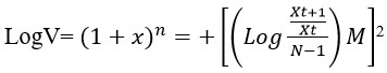
Where,

X_t is the area, production, and productivity of rubber in the year “t”;

Log V is the series’ logarithmic variance;

N is the number of years;

m is the mean of the difference between logs of X_t+1 and X_t.

Model specification

For achieving the goal of how the climatic factors such rainfall and temperature and area of rubber is impacting the rubber production in Kerala- district wise, the present study has used panel ARDL model. Similar panel ARDL model were utilised by Reshma et al.²⁸ The given below equation were employed.

Where,

Pr_it  = Productivity

Ar_it = Area under production

Rn_it = Rainfall

Tem_it = Temperature

‘t’ indicates ‘time’, ‘i’ indicates ‘observation’ and ‘f’ indicates ‘function’.  Equation (5) can be derived from equation (4).

The major research question addressed in this study is: Is the productivity of rubber cultivation district-wise impacted by the variables given above? How it impact the productivity of rubber? Existing research has made contradictory results. For instance, Mesike and Esekhade²⁹ have found that rainfall has a negative impact on rubber cultivation in Nigeria. In the research focusing on Thailand, Sangchanda et al.³⁰ found a significant positive impact of rainfall on the rubber cultivation. Whereas Nguyen and Dang³¹ found an long- term association which is positive between the rubber and temperature. However, there is a lack of research on the effect of climatic factors on the rubber productivity in Kerala, especially a district-wise analysis. Employing the data from 2003 to 2020, the present research attempts to address this gap and to give an idea about the factors affecting the productivity of rubber in Kerala.

Unit root test

The stationarity of the variables included in the study is tested using unit root tests.³²  The first-generation unit root tests used in the current study were the Im, Pesaran, and Shin (IPS) tests, which were introduced by Im et al.,³³ and the LLC (Levin, Lin, and Chu) tests, introduced by Levin et al.³⁴ The second-generation unit root tests, CIPS and CADF developed by Pesaran³⁵ was  also used.

Panel cointegration

The Pedroni panel cointegration test is employed for testing whether the cointegration exists or not. Pedroni³⁶ came up with two different test such as within- dimension and between dimension. If the p-value for each of these data points is below the specified significance threshold, the alternative hypothesis indicating the presence of cointegration is accepted.

Panel ARDL Approach

In the current study, the production of rubber is associated to climatic variables including rainfall, temperature and area. The empirical model states that rubber productivity is a function of these climatic factors and the area under rubber cultivation. For finding the association among the variables, the current research uses the following equation.

The coefficients that measure the influence of explanatory factors on the dependent variable are α₁ to α₃, with α₀ serving as the model’s intercept. Furthermore, to avoid autocorrelation and heteroskedasticity, we translate our model to logarithmic form.³⁷

Panel ARDL was used in the current investigation. The main argument in favour of employing the panel data is that only a minor information is forgone while conducting an analysis.³⁸ The issue of heteroscedasticity can be avoided in panel data.³⁹ Moreover, if the problem of lack of data arise, and if the variables are integrating in different orders I (0) and I (1), then panel method is most suitable. The association between production and its effecting variables are expressed as the equation given below.

In ARDL form, this can be expressed as given below.

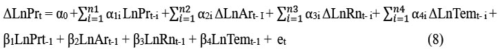
et is the white noise error term, Δ is the initial difference between the variables, and α0 is a drift component. The coefficients from α_1i to α_4i in equation (8) indicate that there is a correlation between short and long-term associations, as indicated by the coefficients from β₁ to β₄. The ARDL model in the error correction form can be represented as follows.

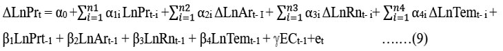
Where ℽ indicates the extent to which the values are adjusted to the previous year shock and error correction are the residual based on equation (9).

Results

Compound Growth Rate- Kerala

Significant trends and changes in Kerala’s rubber cultivation may be seen in the compound annual growth rate (CAGR) while taking into consideration the area under rubber, production and productivity rubber plantations throughout the three different periods from 2003 to 2021. Different dynamics affected by climatic, economic, and policy issues are reflected each time (table 2)

Table 2: Outcome of CAGR

Time Period	Area	Production	Productivity
Period I (2003-04 to 2008-09)	1.3171%	3.0268%	-33.350%
Period II (2009-10 to 2014-15)	0.7639%	-6.2023%	-3.000%
Period III (2015-16 to 2020-21)	-0.0057%	1.9494%	-0.5306%

 Instability analysis of rubber cultivation in Kerala

The stability of rubber cultivation in Kerala is examined in Table 2 for three different periods: Period I (2003–04 to 2008–09), Period II (2009–10 to 2014–15), and Period III (2015–16 to 2020–21). Using important statistical metrics, including the CII, CDVI, and the CV, the instability analysis were undertaken. Each of these indices measures the degree of instability: CII provides a weighted average to measure instability, often used in agricultural research to see how much a variable changes over time; CDVI adjusts the CV by considering how well a trend line fits the data (looking at trends instead of random changes); and CV measures how one variable vary in relation to each other.

Table 3: Instability analysis – Kerala

Time Period/Variables		Area	Production	Productivity
Period I (2003-04 to 2008-09)	Mean	497537.1667	733693.6667	1477.8333
	Std	16068.0583	51152.8343	56.2403
	Adj.  R2	0.9731	0.7831	0.3868
	CV (%)	3.2295	6.9720	3.8056
	CDVI	0.5297	3.2470	2.9800
	CII	38.0005	39.5036	38.2239
Period II (2009-10 to 2014-15)	Mean	539491.3333	711833.3333	1409.8333
	Std	9075.2192	114605.5098	117.7411
	Adj.  R2	0.9265	0.4075	0.1557
	CV (%)	1.6822	16.1000	8.3514
	CDVI	0.4561	12.3929	7.6738
	CII	37.4175	43.9354	40.1996
Period III (2015-16 to 2020-21)	Mean	551000.8333	507596.6667	911.5000
	Std	212.7538	41206.5094	68.9137
	Adj.  R2	-0.2285	-0.2167	-0.2333
	CV (%)	0.0386	8.1180	7.5605
	CDVI	0.0428	8.9544	8.3962
	CII	36.8059	40.0039	39.7561

Impact of climatic factors – Rainfall and Temperature on Rubber Productivity

Cross- Sectional Dependence Test

CDS test reveals a strong cross-sectional dependence between the variables used in the present study. The coefficient value of CD statistics shows that values are highly significant, suggesting that they are not independent between the cross-sectional units. The values of CD statistics are 12.61, 11.47, 15.63, 5.36 for production, area, rainfall, and temperature.

Slope Homogeneity Test

The outcome of the Pesaran and Yamagata⁴⁰ slope homogeneity  are shown in Table 4. The value of the Δ statistic is high, positive and significant. Hence, the alternative hypothesis of heterogeneity is accepted.

Table 4: Slope Homogeneity test result

Test	Δ statistic	P- value
͠Δ test	14.536	0.032
͠Δ adj test	18.496	0.029

Panel unit root test

The results of the panel unit root tests are given in Table 5.

Table 5: Panel Unit Root

Variables	Levin- Chu		CIPS		CADF		Decision
	I (0)	I (1)	I (0)	I (1)	I (0)	I (1)
LnPr	-1.451(0.012)	-4.215***(0.002)	-3.518***(0.009)	-7.185***(0.034)	-1.265***(0.003)	-8.139***(0.000)	I(0)
LnAr	-1.741(0.073)	-3.125***(0.005)	-7.952(0.451)	-9.456***(0.003)	0.541(0.321)	-7.911***(0.000)	I(1)
LnRn	-2.415***(0.002)	-8.632***(0.020)	-2.841***(0.001)	-4.256***(0.002)	-3.174***(0.000)	-8.741***(0.003)	I(0)
LnTem	-1.521(0.081)	-4.521***(0.005)	-8.312(0.332)	-8.519***(0.005)	0.151(0.851)	-6.133***(0.000)	I(1)

Note: *** indicates the significance

Panel cointegration

Results of cointegration test developed by Pedroni is displayed in table 6. This was undertaken to confirm the long-run association between the selected variables. Individual and common auto-regressive coefficients were evaluated.

Table 6: Outcome of Cointegration test

Common AR coefs. (within- dimension)
	Statistic	Prob.	Weighted Statistics		Prob.
Panel v-statistic	-1.84202	0.80012	-0.74321		0.85212
Panel rho- statistic	-2.41212	0.89321	-1.39561		0.90213
Panel PP- Statistic	-8.23451	0.00071	-5.10223		0.00014
Panel ADF- Statistic	-4.69445	0.00019	-4.36962		0.00006
individual AR coefs. (between dimension)
	Statistic			Prob.
Group rho- statistic	-4.36963			0.6123
Group PP- Statistic	-8.51998			0.0001
Group ADF- Statistic	-9.51967			0.0000

Panel ARDL

Using the panel ARDL method, the present investigation found the effect of independent variables such as LnAR, LnRn, and LnTem on the endogenous variable LnPr in both the long and short term. Table 7 display the outcome of long- term panel ARDL.

Table 7: Result of long term estimation- Panel ARDL

Variables	Coefficient	t-statistic	Probability
LnAr	0.3816	4.0251	0.012
LnRn	0.3578	2.7895	0.003
LnTem	-0.1811	2.0012	0.001

 Panel ARDL method outcome in the short run  have been displayed in Table 8. The error term coefficient value in any model indicates the extent to which the current year can adjust to the previous year’s uncertainties and shocks.^{28, 41} In the current study the value of the error term is -0.5217.

Table 8: Result of Short term- Panel ARDL

Variables	Coefficient	t-statistics	Prob.
COINTEQ01	-0.5217	-6.324	0.003
DLnAr	0.2302	2.623	0.058
DLnRn	0.3412	1.336	0.004
DLnRn(-1)	0.3741	1.202	0.012
DLnTem	0.2812	6.236	0.030
C	-20.362	-12.634	0.001

 Discussion

Compound annual growth rate of rubber cultivation in terms of area, production and productivity were examined by dividing into three period. Period I (2003–04 to 2008–09): Production rose at 3.026 percent annually during this first period, while the area under rubber cultivation expanded at a positive CAGR of 1.3171 percent. However, with a negative growth rate of -33.350 percent, productivity fell precipitously and unexpectedly. This contradictory pattern—increasing area and output but decreasing productivity—indicates that land coverage, not increases in per-hectare yield. This can be substantiated with several reason. First, farmers cultivate rubber in additional areas in the early 2000s due to high rubber prices, including marginal and sub-optimal lands. ¹ mentioned this in the paper analysing the history of Kerala’s rubber cultivation. He further reported that a shortage of rubber and increased demand during the late 1990s have led the existing cultivators to increase production to earn more profit. However, productivity did not increase in the same manner. Second, the reduction in yield per unit area may have been caused by inadequate replanting techniques, a lack of acceptance of high-yielding seeds, and limited technical developments. Additionally, even as farmers increased cultivation, Kerala during that period witnessed unpredictable rainfall patterns and sporadic pest and disease outbreaks, negatively impacting rubber yield. This was reported in a study by Thomas.⁴²

Period II (2009–10 to 2014–15): During this second period, the area under rubber plantation grew at a slower pace of 0.7639 percent. Production saw a sharp decline, registering a  negative CAGR of -6.2023 percent. Despite being negative, productivity increased compared to Period I, declining by a comparatively lower amount at -3.000 percent. There are several reasons for this decline. Global economic problems, including the 2008 financial crisis and competition from synthetic rubber, were the leading causes of the significant fluctuation in international rubber prices. Reduced production resulted from farmers’ reluctance to continue or expand rubber cultivation as prices declined. This was mentioned in a study by Karunakaran,¹⁵ since most rubber producers in Kerala are small-scale operators.

Therefore, any financial limitations, price swings, or technological lag would significantly impact the cultivators. Farmers, particularly smallholders, were deterred from sustaining productivity by labour shortages and the rising expense of tapping operations. In the prevailing rubber smallholding industry, the lack of workers, particularly rubber tappers, has been increasingly problematic in recent years for several reasons, including the following: (a) the increase in smallholders’ rubber-operated land and the corresponding increase in rubber-tapped land; (b) the reluctance of younger generations to pursue rubber tapping as a business venture; (c) the comparatively low presence and active involvement of women in rubber tapping and associated activities; and (d) the ageing of the current tapping workforce.^{11, 43-44}

Period III (2015–16–2020–21): With an almost insignificant negative CAGR of -0.0057 percent, the area under rubber cultivation affected adversely. While productivity saw a slight fall of -0.5306%, production growth rebounded significantly, with a positive CAGR of 1.9494%. Improved tapping techniques, a greater use of disease-resistant cultivars, and better farm management techniques all helped to stabilise yield levels as the government of Kerala has increased the budget allocated for plantations with the aim of reviving plantation industries.⁴¹

With a CV of 3.23 percent, a CDVI of 0.5297, and a CII of 38.00, the average area under rubber cultivation during Period I (2003-04 to 2008-09) was 497,537 hectares. These values show a moderate degree of variability in the area under cultivation. Increase in area was very constant throughout this time, despite minor fluctuations, according to the comparatively low CV and CDVI. Production indicated considerable inconsistency with a CV of 6.97%, CDVI of 3.247, and CII of 39.50. The higher value of CV and CDVI suggests that external variables such as diseases, market forces, and climatic fluctuations had a greater impact on production. Productivity was consistent, as indicated by its CV of 3.80%, CDVI of 2.980, and CII of 38.22.

During Period II (2009–10), the value of CDVI, CII, and CV for area were 0.4561, 37.41, and 1.68 percent with a average area of 539,491 hectares. Compared to Period I, this decrease in variability indicates that rise in area under cultivation became more consistent. The production situation, however, deteriorated significantly: the CII increased to 43.93, the CDVI to 12.39, and the CV to 16.10%, all indicating considerable instability. This implies that even while the area has increased, production was highly variable, mostly due to unpredictable weather patterns, insect infestations, or variations in tapping intensity. Compared to Period I, productivity also saw more volatility, with a CV of 8.35%, a CDVI of 7.67, and a CII of 40.19. Small rubber farmers face low yield, subpar processing, and a weak marketing strategy. Due to the large number of smallholdings, the industry is susceptible to price swings, middleman exploitation, etc., which can contribute to instability.³³

The mean area expanded slightly to 551,000 hectares in Period III (2015–16 to 2020–21). However, the CV fell to a very low 0.0386 percent, with a CDVI of 0.0428 and a CII of 36.80. These extremely low numbers suggest that the area used for rubber production has stabilised, which may result from the state government’s stabilisation or growth strategies. Production’s CV, CDVI, and CII were 8.12 percent, 8.95, and 40.00, respectively, indicating moderate instability. Better management techniques may cause decreased production variability. With a CV of 7.56 percent, a CDVI of 8.39, and a CII of 39.75, productivity exhibited significant fluctuation, mirroring production patterns. Production swings were comparatively limited compared to Period II, even though they remained concerning.

Further, the study also determined the impact of rainfall and temperature on rubber productivity using the panel data across all the 14 districts of Kerala. First, cross- sectional dependence test were conducted which indicates that any variation in one element lead to variation in the value of the other variables also. The result of slope homogeneity test further shows that slopes of this panel model are not even between the cross-sectional. Then the panel unit root test were undertaken. Because of the high p-value (more than 0.05), the variables such as area (LnAr) and temperature (LnTem) indicate non-stationarity at the level. However, after transforming the variable into the first difference, the stationarity is achieved. Hence, for analysis, the variables such as area (LnAr) and temperature (LnTem) are converted into first differences for further examination. Whereas, the variables such as production (LnPr) and rainfall (LnRn) become stationary at level.

Following, panel cointegration were undertaken. Results of v-statistic and rho-statistic shows an inverse value, indicating contradicting evidence for a long-term connection, even if they are statistically insignificant. However, the no cointegration hypothesis is firmly disproved by the panel cointegration outcome. Since the values are negative for both Group PP and Group ADF, we fail to accept the null hypothesis.

Then panel ARDL test including the long and short term impact. Area (LnAr) has a positive effect on the productivity of rubber (LnPr) in the long term, with a coefficient value of 0.38 indicating that 1 percent rise in the LnAr would increase the yield of rubber by 0.38 percent which was in line with the existing literature, such as Datta et al.⁴⁵ This can be connected to the benefits of scale, since greater cultivated areas promote more effective use of inputs, mechanisation, and scientific agricultural methods. Rainfall (LnRn) is a contributing factor to the rise in productivity of rubber, as seen by the positive and significant long-term coefficient of LnRn. A 1 percent rise in rainfall leads to 0.35 percent increase in productivity. Sufficient rainfall promotes nutrient absorption, increases soil moisture, and supports the physiological processes required for strong tree development. Higher yields are the result of improved latex flow and less stress on the trees caused by this favourable water availability. Therefore, regions with regular and well-distributed rainfall are more likely to observe enhanced rubber productivity. These findings were supported by Sangchanda et al.,³⁰ and Mesike and Esekhade.²⁹

However, temperature (LnTem) has a negative effect on rubber productivity (LnPr) with a coefficient value of -0.18. The reason behind this is because rubber trees are extremely vulnerable to drastic changes in temperature. High temperatures can impair latex production by causing heat stress, increasing evapotranspiration, and decreasing soil moisture. Long-term high temperatures may also interfere with rubber tree physiological functions, including photosynthesis and nitrogen absorption, which would reduce productivity. This was in line with the outcome of Ling et al.,⁴⁶ In the short term, error term indicates that the current year’s degree of adjustment to the previous year’s shock are by 52.17 percent. And LnRn (rainfall) and LnTem (temperature) has a favourable effect on the productivity (LnPr) with values of 0.34 and 0.28. However, the area (LnAr) is positive, but it is insignificant.

Conclusion

The current study examined Kerala’s rubber cultivation’s development trends and determinants from time period 2003 to 2021- a time when the industry saw significant structural changes. The study divided the analysis into three phases: 2003–2008, 2009–2015, and 2016–2021. It used econometric modelling using a Panel Autoregressive Distributed Lag (ARDL) approach, the Compound Annual Growth Rate (CAGR), and instability indices (CV, CDVI, and CII) to evaluate changes in area, production, and yield. The results show that, even while productivity has somewhat stabilised in recent years, rubber cultivation area and production have been declining, especially after 2009. The instability study revealed notable variations, particularly in output and productivity during the second phase, while the CAGR analysis demonstrated a declined growth rate in area and productivity throughout periods. These trends suggest that Kerala’s rubber sector is becoming more vulnerable and unpredictable, which is probably being made worse by pressures from the environment and the economy.

Deeper understanding of the connection between temperature and rainfall, two climatic factors, and rubber productivity was made possible by the econometric study. The Panel ARDL data throughout time verified a statistically significant and favourable correlation between rainfall and both area under cultivation and production. However, temperature had a markedly negative influence, highlighting how rising temperatures have a negative effect on rubber yield. All three factors—temperature, rainfall, and area—improved production in the short term, while area’s influence was statistically negligible. According to this differentiation between short- and long-term dynamics, continuous climatic trends—in particular, temperature rise—present a significant effect the regions rubber production over the long run. Kerala’s agriculture and climatic adaptation policies would be significantly impacted by these findings. First, the rubber industry urgently needs to encourage climate-resilient farming methods. Given the detrimental long-term effects of temperature on production, climate change may further negatively affect the economic viability of rubber cultivation in the absence of intervention, particularly in areas more susceptible to heat stress. Second, while rainfall boosts production, investments in water management infrastructure, including check dams, rainwater gathering units, micro-irrigation systems, and better drainage, are necessary to provide a steady and adequate water supply. These methods will guarantee more consistent latex output all year round in addition to lessening water stress during dry times.

Furthermore, the study underscores the continuous need of preserving or even extending the area under rubber cultivation whenever environmentally and economically possible. Larger agricultural fields are frequently connected with more effective resource usage, better access to mechanisation, and enhanced institutional support. The observed stalling and eventual reduction in cultivated area over the research period, however, may be a reflection of more general problems, including diminishing profitability, a lack of workers, and competition from other land uses or crops. Labour scarcity, driven by rural outmigration and the rising cost of wages, has increased the dependence on hired workers and mechanisation. Addressing this issue will require greater promotion of mechanised tapping, skill development programmes for local youth, and farmer cooperatives that can pool labour resources. Supportive government policies such as minimum support prices, crop insurance, and incentives for mechanisation can also help farmers overcome labour constraints. In addition, strengthening cooperative and cluster-based structures will enhance collective bargaining power, ensure economies of scale, and make credit and technology more accessible. Smallholders can also get access to technology and capital, develop collective resilience, and realise economies of scale by supporting cooperative and cluster-based structures. It must serve as the central hub for developing and carrying out credit, insurance, and price stability policies. It is recommended that the PSF programme be made mandatory or restructured so that many farmers may participate. This might be accomplished by integrating PSF with finance, insurance, replanting planting subsidies, etc.

Acknowledgement

The authors would like to thank the authorities of the institutions that the authors belong to for granting the academic freedom and help in publishing this paper. Our thanks are due particularly to the library of Avinashilingam Institute for Home Science and Higher Education for Women, Coimbatore for providing access to data for this study.

Funding Sources

The   author(s) received   no   financial   support   for   the   research,   authorship,   and/or publication of this article.

Conflict of Interest

The authors do not have any conflict of interest

Data availability Statement

The datasets used and analysed during the current study are available from the author, Ms Soumya Sahadevan, upon reasonable request.

Ethics Statement

This research did not involve human participants, animal subjects, or any material that requires ethical approval.

Informed Consent Statement

This study did not involve human participants, and therefore, informed consent was not required.

Permission to reproduce material from other sources

Not Applicable

Author contributions:

Sowmya Sahadevan: Conceptualization, Methodology, Writing, Data Collection, Analysis

Malarvizhi Vaithiyanathan: Visualization, Supervision

Reference

1. Sarkar, S. Rubber plantation: A new hope for rural Tribals in Tripura. International Journal of Plant Sciences. 2011: 6(2): 274-279.
2. Min, S., Waibel, H., Cadisch, G., Langenberger, G., Bai, J., & Huang, J. The economics of smallholder rubber farming in a mountainous region of Southwest China: Elevation, ethnicity, and risk. Mountain Research and Development. 2017: 37(3):  https://doi.org/10.1659/mrd-journal-d-16-00088.1
   CrossRef
3. FAOSTAT Statistics Division. 2017. https://faostat3.fao.org/faostat-gateway/go/to/download/Q/QC/E
4. Sinumon, T. G., & Mahalakshmi K. Study on the Problems faced by the rubber growers in Kerala. International Journal of Management (IJM). 2020: 11(12): 4032-4038.
5. Jin, S., Min, S., Huang, J., & Waibel, H. Rising labour costs and the future of rubber intercropping in China. International Journal of Agricultural Sustainability. 2021: 20(2): 124-139. https://doi.org/10.1080/14735903.2021.1918482
   CrossRef
6. Longkumer, W., & Sharma, A. Economics of rubber plantation in Mokokchung district. Indian Journal Of Agricultural Research. 2023. https://doi.org/10.18805/ijare.a-6137
   CrossRef
7. Study: Unchecked rubber spread in northeast India threat to native forest. Retrieved November 15, 2022 from http://india.mongabay.com/2018/03/rubber/.
8. Ushadevi, T.V. and Jayachandran, V.N. Socio-economic profile of rubber tappers in the smallholding sector: A study at Kanjirappally Panchayat. Kerala Research Programme on Local Level Development, Centre for Development Studies, Thiruvananthapuram. 2001: 64.
9. Adikari, S., & Sharma, A. Marketing pattern of rubber plantation in Tripura. International Journal of Current Microbiology and Applied Sciences. 2018: 7(06): 847-853.  https://doi.org/10.20546/ ijcmas.2018.706.099
   CrossRef
10. Muralidharan, V. K. A study on the problems and prospects of small rubber cultivators in Pattambi area. International Education & Research Journal [IERJ]. 2015: 1(5): 112-115.
11. Kadavil, T. Tapping labour shortage and dilemmas in policy options: The case of rubber smallholder sector in Kerala. SSRN Electronic Journal. 2012. https://doi.org/10.2139/ssrn.2410142
    CrossRef
12. Nair S, M. K. Rural labour market in Kerala: Smallholder agriculture and labour market dynamics. Economic and Political Weekly. 1999: 32(35): 45-52.
13. Viswanathan, P. K. Labour shortage in rubber sector in Kerala. Globalisation, Development and Plantation Labour in India. 2016: 196-233. https://doi.org/10.4324/9781315620510-8
    CrossRef
14. Viswanathan, P.K., George, Tharian, K. & Joseph, T. Informal labour market and structural devolution. Economic and Political Weekly. 2003: 38(31): 3277-3281.
15. Karunakaran, N. Volatility in price of rubber crop in Kerala. Journal of Krishi Vigyan. 2017: 5(2): 160.  https://doi.org/10.5958/2349-4433.2017.00035.6
    CrossRef
16. Mardhiyah, A. Rubber production marketing strategy. Proceedings of the International Conference of Science, Technology, Engineering, Environmental and Ramification Researches. 2018: 1736-1740.  https://doi.org/10.5220/0010097517361740
    CrossRef
17. Government of Kerala. A Compendium of Agricultural Statistics: Kerala 2023. Karshika Keralam – Department of Agriculture Development and Farmers’ Welfare. 2023 https://keralaagriculture.gov.in/ wp-content/ uploads/2023/04/AGRICULTURAL-STATISTICS-2023.pdf
18. India Meteorological Department. (2025). India Meteorological Department. India Meteorological Department. https://mausam.imd.gov.in
19. Dandekar, V. M. Introduction seminar on data and methodology for the study of growth rates in agriculture. Indian Journal of Agricultural Economics. 1980: 35(2): 1-12.
20. Singh, I. J., & Rai, K. N. Regional variations in agricultural performance in India. Indian Journal of Agricultural Economics. 1997: 52(3): 374-377.
21. Wani, B., Kaspate, R., & Memane, S. R. Growth and instability in area, production and productivity of major cash crops in India. Ecology, Environment and Conservation. 2024:  30(02): 858-864.  https://doi.org/10.53550/eec.2024.v30i02.073
    CrossRef
22. Larson, D. W., Jones, E., Pannu, R., & Sheokand, R. Instability in Indian agriculture—a challenge to the Green Revolution technology. Food Policy. 2004: 29(3): 257-273.  https://doi.org/10.1016/j. foodpol.2004.05.001
    CrossRef
23. Cuddy ,J. A., & Della-Valle P. A. Measuring the instability in time series data. Oxford Bulletin of Economics and Statistics. 1978: 41(3) :247-248.
    CrossRef
24. Jambhulkar, N. N., Mondal, B., Bisen, J., Mishra, S. K., & PRADHAN, A. K. Growth and instability analysis of rice production: A district level assessment in Uttar Pradesh and Uttarakhand states of India. The Pharma Innovation Journal. 2023: 12(2): 813- 819.
25. Samal, P., Rout, C., Repalli, S., & Jambhulkar, N. State-wise analysis of growth in production and profitability of rice in India. Indian Journal of Economics and Development. 2018: 14(3): 399. https://doi.org/10.5958/2322-0430.2018.00151.8
    CrossRef
26. Jambhulkar, N. N., Mondal, B., Paul, S., Pradhan, A. K., & Kumar, G. A. Analysis of growth and instability of rice production in Madhya Pradesh, India: A district level study. Journal of Experimental Agriculture International. 2024: 46(10): 316-324. https://doi.org/10.9734/jeai/2024/v46i102953
    CrossRef
27. Kaur, N. and Singhal, K.C. India’s Export Instability. Margin. 1988; 21: 54-61.
28. Reshma V., Pradeesh, K., Mohandas, V. K., & Manikandan, K. Understanding the impact of artificial intelligence on the stock market development in BRICS nations: a panel ARDL method. Theoretical and Applied Economics. 2025: 32(2): 35-52. https://store.ectap.ro/articole/1830.pdf
29. Mesike, C. S., & Esekhade, T. U. Rainfall variability and rubber production in Nigeria. African Journal of Environmental Science and Technology. 2014; 8(1): 54-57. https://doi.org/10.5897/ajest2013.1593
    CrossRef
30. Sangchanda, N., Ayutthaya, S. I., Meetha, S., & Songsri, P. The influence of rainfall on growth of rubber trees in marginal area of Northeast Thailand. Advanced Materials Research. 2013; 844: 7-10. https://doi.org/10.4028/www.scientific.net/amr.844.7
    CrossRef
31. Nguyen, B. T., & Dang, M. K. Temperature dependence of natural rubber productivity in the southeastern Vietnam. Industrial Crops and Products. 2016; 83: 24-30.  https://doi.org/10.1016/j.indcrop.2015.12.019
    CrossRef
32. Joo, B. A., & Shawl, S. Understanding the relationship between foreign direct investment and economic growth in BRICS: Panel ARDL approach. Vikalpa: The Journal for Decision Makers. 2003; 48(2): 100-113. https://doi.org/10.1177/02560909231180078
    CrossRef
33. Im, K. S., Pesaran, M. H., & Shin, Y. Testing for unit roots in heterogeneous panels. Journal of Econometrics. 2003: 15: 53-74. https://doi.org/0.1016/S0304-4076(03)00092-7
    CrossRef
34. Levin, A., Lin, C., & James Chu, C. Unit root tests in panel data: Asymptotic and finite-sample properties. Journal of Econometrics. 2002: 108(1): 1-24. https://doi.org/10.1016/s0304-4076(01)00098-7
    CrossRef
35. Pesaran, M. H. Estimation and inference in large heterogeneous panels with a multifactor error structure. Econometrica. 2006: 74(4): 967-1012. https://doi.org/10.1111/j.1468-0262.2006.00692.x
    CrossRef
36. Pedroni, P. Critical values for Cointegration tests in heterogeneous panels with multiple Regressors. Oxford Bulletin of Economics and Statistics. 1999: 61(s1): 653-670.  https://doi.org/10.1111/1468-0084.0610s1653
    CrossRef
37. Hassan, A. Y., & Mohamed, M. A. Dynamic impacts of economic and environmental performances on agricultural productivity in Somalia: Empirical evidence from ARDL technique. Cogent Food & Agriculture. 2024: 10(1). https://doi.org/10.1080/23311932.2024.2369204
    CrossRef
38. Baltagi, B. Econometric analysis of panel data. John Wiley & Sons. 2008.
39. Ahn, S. C., Lee, Y. H., & Schmidt, P. Panel data models with multiple time-varying individual effects. Journal of Econometrics. 2013: 174(1): 1-14. https://doi.org/10.1016/j.jeconom.2012.12.002
    CrossRef
40. Pesaran, M. H., & Yamagata, T. Testing slope homogeneity in large panels. SSRN Electronic Journal. 2005. https://doi.org/10.2139/ssrn.671050
    CrossRef
41. Vattekkad, R., Krishnan, M., Krishna, R., Sahadevan, S., Krishna, D., & Renuka, D. Evaluating the influence of climatic and non- Climatic factors on horticultural production in India- An ARDL approach. Current Agriculture Research Journal. 2025: 13(1); 362-375.  https://doi.org/10.12944/ carj.13.1.36
    CrossRef
42. Thomas, C. A. Small rubber growers and rubber producers’ societies in Kerala[Doctoral dissertation]. 2004
43. Government of Kerala. Report of Working Group on Plantation Economy. Industry and Infrastructure Division, Kerala. 2022.  https://spb.kerala.gov.in/sites/default/files/inline-files/Plantation% 20Layout %409.5.23.pdf
44. Shanmugavadivu N., & Kavitha, K. R. A Study on the Problems of Small Rubber Growers with Special Reference to Kodanchery Panchayath, Kozhikode District. AEIJMR. 2015: 3(10).
45. Datta, H., Debnath, H., & Shil, P. Production and productivity of natural rubber: A study on growth-trends of rubber plantation in Tripura. International Journal of Management. 2019; 10(4).  https://doi.org/10.34218/ijm.10.4.2019.011
    CrossRef
46. Ling, Z., Shi, Z., Gu, S., Wang, T., Zhu, W., & Feng, G. Impact of climate change and rubber (Hevea brasiliensis) plantation expansion on reference evapotranspiration in Xishuangbanna, Southwest China. Frontiers in Plant Science. 2022: 13. https://doi.org/10.3389/fpls.2022.830519
    CrossRef