The Impact of Climate Change on Wheat Production in Punjab: A Time Series Approach

Introduction

The state of Punjab, often referred to as the “Granary of India,” has long been a significant contributor to the country’s agricultural output, particularly in wheat production. With its fertile soil, well-irrigated land, and advanced agricultural practices, Punjab has played a crucial role in ensuring national food security. However, the region is now confronting a formidable challenge in the form of climate change, which poses a serious threat to its agricultural landscape, including the production of staple crops such as wheat.¹

Climate change is a global phenomenon marked by long-term shifts in weather patterns, temperature extremes, and altered precipitation levels. Scientific consensus holds that human activities, primarily the emission of greenhouse gases are driving these changes. In Punjab, the effects of climate change on wheat production are becoming increasingly evident, influencing the state’s agricultural economy and, by extension, the country’s overall food security.² One of the most noticeable manifestations of climate change in Punjab is the alteration of traditional weather patterns. Shifts in temperature and precipitation have disrupted the finely tuned agricultural calendar that farmers have relied upon for generations. Rising temperatures during critical stages of wheat growth, for instance, can negatively affect yields by altering processes such as flowering and grain filling.³ Additionally, unpredictable and extreme weather events such as unseasonal rainfall and heat waves have become more frequent, further complicating agricultural planning and operations.⁴

Water availability in Punjab is also undergoing substantial changes due to climate change. The region depends heavily on the Indus River and its tributaries for irrigation, and variations in precipitation are influencing both the timing and volume of water flow. Altered snowmelt patterns from Himalayan glaciers, which feed these rivers, may lead to fluctuations in water availability during the crucial planting and maturation stages of wheat cultivation.

Moreover, climate change has ushered in new dynamics in pest and disease prevalence. Warmer temperatures can create favourable conditions for the proliferation of pests and diseases that were previously kept under control by colder winters.^{5, 6} This has contributed to a rise in pest infestations, posing a direct threat to wheat crops and necessitating modifications in pest management strategies.⁷

The interdependent relationship between Punjab’s agricultural productivity and the climate is now under significant strain as the impacts of climate change continue to unfold. The objective of this study is to conduct an econometric analysis of the multifaceted implications of climate change on wheat production in Punjab, recognizing the interconnected nature of climatic factors and agricultural outcomes. The study aims to identify emerging trends and patterns that illustrate the evolving climate scenario in the region. Understanding how farmers are adapting to these changes and the challenges they encounter is essential for formulating effective policy interventions and support mechanisms.

This paper is organized into five sections. The first section provides the introduction, followed by the literature review, data and methodology, results and discussion, and finally, conclusions and policy implications.

Review of Literature

This review of literature examines existing research on the impact of climate change on wheat production in Punjab, India, using an econometric approach to understand this relationship. Climate change is altering global temperature and rainfall patterns, with significant implications for agricultural productivity. Reports by the Intergovernmental Panel on Climate Change (IPCC, 2014) highlight the growing frequency of extreme weather events including droughts, heat waves, and erratic rainfall that directly affect crop growth and yields. Studies by researcher^8-10 further document the negative effects of rising temperatures on wheat output, emphasizing the importance of considering regional differences and adaptive responses.

Punjab, often referred to as the “Granary of India,” remains a key contributor to national wheat production. Its agricultural strength is supported by fertile soils, an extensive irrigation system, and high-yielding crop varieties. However, climate change poses a serious threat to this long-standing agricultural base. Research¹¹,¹² highlights the vulnerability of wheat production in Punjab to climatic variability, with broader implications for food security and rural livelihoods.

Econometric methods provide valuable tools for analysing the relationship between climate variables and agricultural outcomes. Studies such as^13,14 use panel data models to examine how temperature and precipitation influence wheat yields while accounting for soil characteristics, farming practices, and socio-economic factors. Their findings stress the importance of incorporating both spatial and temporal variations in climate data to capture localized effects accurately.

Addressing the challenges posed by climate change requires effective adaptation and mitigation strategies. Agronomic interventions such as heat-tolerant wheat varieties and water-efficient irrigation technologies offer promising solutions for reducing climate-related risks.¹⁵ Policy measures, including crop insurance schemes and enhanced agricultural extension services, can further support farmers in managing climate shocks.¹⁶

This research paper aims to fill an important gap in the existing literature by examining the long-term impact of climate change on wheat production in Punjab over the period 1990 to 2021. While many studies have explored the connection between climatic factors and agricultural performance, comprehensive analyses focusing on this specific timeframe and region remain limited. By employing the Autoregressive Distributed Lag (ARDL) model and associated diagnostic tests, this study seeks to provide a deeper understanding of the long-run effects of climate change on wheat yields in Punjab.

Materials and Methods

The research aimed to examine the impact of climate change on wheat production in Punjab, India, for the period 1990–2021. To conduct the time-series co-integration analysis, the study employed the Autoregressive Distributed Lag (ARDL) model, following methodological refinements.^17-19

To determine the order of integration of the variables, stationarity tests—namely the Augmented Dickey–Fuller (ADF) and Phillips–Perron (PP) unit-root tests—were applied in accordance with the procedures outlined.²⁰ Lag length selection for the ARDL bounds test was based on the Schwarz Information Criterion (SIC), ensuring an optimally specified model. When initial conditions for the dependent variable were not met, a modified ARDL bounds test employing surface regression was utilized.

To address potential heteroskedasticity issues, all variables were expressed either in percentage terms or transformed into natural logarithms. Model stability diagnostics were also conducted to evaluate the consistency and reliability of the estimates, as detailed in the methodology. Figure 1 presents a visual summary of the stability tests performed. Through this rigorous methodological framework, the study sought to generate robust evidence on the relationship between climate change and wheat production in Punjab, offering meaningful insights for agricultural policy formulation and climate-adaptation strategies.

Model specification and functional form

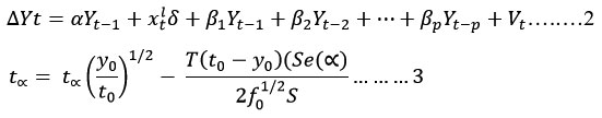
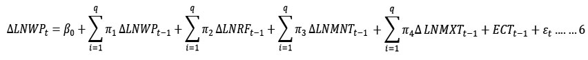
To elucidate the relationship between wheat production, rainfall, minimum temperature, and maximum temperature, we employ the following equation:

In this context, LNWP_t represents the natural logarithm of wheat production as the dependent variable. The variables LNRF_t, LNMNT, and LNMXT denote the natural logarithm of rainfall, minimum temperature, and maximum temperature, respectively. The parameters α, β, 1, β, 2, and β, 3 represent the constant and different elasticities, while ε(t) represents the error terms in the equation.

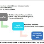Figure 1: Presents the visual summary of the stability test performedClick here to view Figure

Lag lengths of 1 and 3 are determined to be appropriate. To assess serial correlation in the error term, the Augmented Dickey–Fuller (ADF) test is utilized, incorporating lagged differences of the dependent variable. The ADF unit root equation is expressed in (2), while the formula for the Phillip–Perron unit root test, serving the same purpose, is presented in (3).

The equation representing the ARDL bounds testing in the model is articulated as follows in (4),

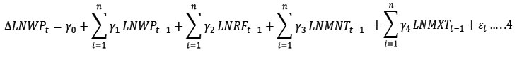
The Long-run and Short-run Autoregressive Distributed Lag (ARDL) approach, as outlined by ²¹ is presented as follows. Equation (5) describes the long-run ARDL model to be estimated.

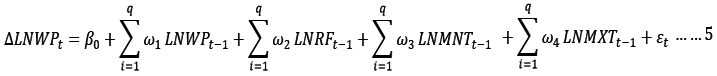
In Equation (5), ω denotes the long-run variance of variables. For the short-run ARDL model incorporating the error correction term, the formulation is articulated as follows:

Data specification

This research relies on secondary data sourced from the IMD (India Meteorological Department) and the RBI (Reserve Bank of India) handbook Indicator database. The dataset spans a time series of 31 years, as detailed in Table 1. The primary variable of interest is the natural logarithm of annual wheat production, serving as the dependent variable. The independent variables encompass rainfall, maximum temperature, and minimum temperature. 

Table 1: Variable names and description

Symbol	Variable Name	Measurement Unit	Source
WP	Wheat  production	Wheat  production (Million tonnes)	RBI
RF	Rainfall	Rainfall (Centimetre)	RBI
MNT	Minimum temperature	Minimum temperature (Kelvin)	IMD
MXT	Maximum temperature	Maximum Temperature (Kelvin)	IMD

Sources: IMD, RBI Handbook

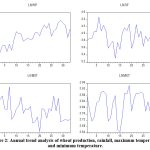Figure 2: Annual trend analysis of wheat production, rainfall, maximum temperature and minimum temperature.Click here to view Figure

Results and Discussion

To analyse the trends depicted in Figure 2 for the variables Wheat Production in Million Tonne, Rainfall, Minimum Temperature, and Maximum Temperature over the years, the use of a trend line can be beneficial. A trend line visually represents the general direction or tendency of the points in Figure 2 over time. The Wheat Production trend line displays a fluctuating pattern with some variability across the years. Although there is variability, a visual examination suggests a potential overall upward trend from 1990 to 2021. Utilizing a trend line would capture and quantify this pattern more effectively. The Rainfall pattern in Figure 2 exhibits variability, and a trend line could reveal the overall direction. From the early 1990s to the mid-2000s, there appears to be a gradual increase, followed by a period of fluctuations. Towards the end of the dataset, a slight increase is noticeable, and a trend line would offer a clearer understanding of the trend. The Minimum Temperature in Figure 2 demonstrates a relatively stable trend over the years with some fluctuations. A trend line would aid in identifying any gradual increase or decrease in minimum temperature over the provided time span.

Regarding the Maximum Temperature in Figure 2, fluctuations are observed, suggesting potential periods of increase and decrease. A trend line would be instrumental in identifying the overall direction of change in maximum temperatures over the years.

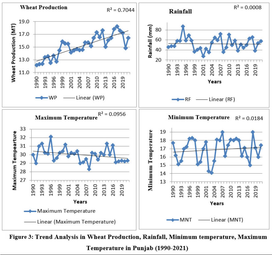Figure 3: Trend Analysis in Wheat Production, Rainfall, Minimum temperature, Maximum Temperature in Punjab (1990-2021).Click here to view Figure

Note: The figure illustrate the long term trends in climatic variables and wheat production used ARDL analysis.

Table 2: Descriptive Statistics

	LNWP	LNRF	LNMXT	LNMNT
Mean	2.71	3.93	3.40	2.82
Median	2.72	3.93	3.40	2.84
Maximum	2.90	4.46	3.47	2.94
Minimum	2.50	3.31	3.34	2.65
Std. Dev.	0.12	0.25	0.03	0.08
Skewness	-0.30	-0.24	0.41	-0.50
Kurtosis	2.17	2.82	2.92	2.20
Jarque-Bera	1.44	0.36	0.93	2.27
Probability	0.49	0.83	0.63	0.32

Source: Author’s Calculation

Table 2 provides descriptive statistics for four variables: LNWP, LNRF, LNMXT, and LNMNT. The mean values, representing the average levels of the variables, are 2.71 for LNWP, 3.93 for LNRF, 3.40 for LNMXT, and 2.82 for LNMNT. The median values, which signify the middle values of each variable, closely align with their respective means. The data range is depicted by the maximum and minimum values: LNWP ranges from 2.50 to 2.90, LNRF from 3.31 to 4.46, LNMXT from 3.34 to 3.47, and LNMNT from 2.65 to 2.94. Standard deviation, indicating the dispersion of data around the mean, is smallest for LNWP (0.12) and largest for LNRF (0.25). Skewness, measuring distribution asymmetry, is close to zero for all variables, indicating approximately symmetrical distributions. Positive kurtosis values for all variables suggest relatively heavy tails in the distributions. The Jarque-Bera test for normality indicates, based on associated probabilities, that the variables are likely normally distributed.

Table 3: Correlation Dependent and Independent variable

	LNWP	LNRF	LNMXT	LNMNT
LNWP	1.00
LNRF	-0.029	1.00
LNMXT	-0.135	-0.03	1.00
LNMNT	0.100	0.396	-0.215	1.00

Source: Author’s Calculation Eview-10

Table 3 displays a correlation matrix illustrating the pairwise correlations among four variables: LNWP, LNRF, LNMXT, and LNMNT. The diagonal elements, representing the correlation of each variable with itself, are consistently 1.00, as expected. The off-diagonal elements indicate the pairwise correlations between different variables. For instance, the correlation between LNWP and LNRF is -0.029, suggesting a weak negative correlation. Similarly, the correlations between LNWP and LNMXT (-0.135) and between LNWP and LNMNT (0.100) are indicative of weak correlations. The correlation between LNRF and LNMXT is -0.03, indicating a very weak negative correlation, while the correlation between LNRF and LNMNT is 0.39, suggesting a moderate positive correlation. The correlation between LNMXT and LNMNT is -0.215, signifying a weak negative correlation.

Table 4: Unit root test

UNIT ROOT TEST TABLE (ADF)
At Level					At First Difference
	LNWP	LNRF	LNMXT	LNMNT	d(LNWP)	d(LNRF)	d(LNMXT)	d(LNMNT)
t-Statistic	-2.22	-4.28	-4.78	-3.99	-7.17	-8.97	-9.72	-6.02
Prob.	0.20	0.00	0.0005	0.00	0	0	0	0
	n0	***	***	***	***	***	***	***
UNIT ROOT TEST TABLE (PP)
At Level					At First Difference
	LNWP	LNRF	LNMXT	LNMNT	d(LNWP)	d(LNRF)	d(LNMXT)	d(LNMNT)
t-Statistic	-2.06	-4.31	-4.84	-3.83	-9.39	-9.41	-11.28	-14.83
Prob.	0.25	0.00	0.00	0.00	0	0	0	0
	n0	***	***	***	***	***	***	***

Source: Author’s Calculation Eview-10

Table 4 presents the results of the unit root tests, specifically the Augmented Dickey Fuller (ADF) and Phillips–Perron (PP) tests. These tests are widely used in time-series analysis to determine whether a series contains a unit root, which would indicate non-stationarity at the level of LNWP. The t-statistic for LNWP is –2.22 with a p-value of 0.20. Although the null hypothesis is not explicitly stated, the p-value being greater than common significance levels such as 0.05 suggests that the null hypothesis of a unit root cannot be rejected.

In contrast, the t-statistic for LNRF is 4.28 with a p-value of 0.00, which strongly rejects the null hypothesis and indicates that the variable becomes stationary after differencing. Similarly, LNMXT has a t-statistic of 4.78 with a p-value of 0.00, providing strong evidence against the null hypothesis and confirming stationarity after differencing. For LNMNT, the t-statistic of –3.99 with a p-value of 0.00 also indicates rejection of the null hypothesis and suggests that the variable is stationary after differencing. Across all variables, the first-difference t-statistics are more negative than their level values, and the p-values approach zero, providing strong evidence against non-stationarity.

The Phillips–Perron (PP) test results at the level similarly show low p-values for all variables, indicating rejection of the unit-root null hypothesis. At the first difference, the t-statistics become even more negative and the p-values remain near zero, further confirming stationarity. Taken together, the ADF and PP test findings indicate that the variables are stationary after first differencing, supporting the presence of co-integration within the Autoregressive Distributed Lag (ARDL) framework. Accordingly, the ARDL model is employed prior to conducting the bounds test, which identifies both the long-run and short-run relationships between the dependent and independent variables.

Table 5: Bound Test dependent and independent variable

Test Statistic	Value	Significance.	I(0) lower	I(1) Upper
F-statistic	5.29	10%	2.01	3.1
k	3	5%	2.45	3.63
		2.50%	2.87	4.16
		1%	3.42	4.84

Source: Author’s Calculation Eview-10

Table 5 provides essential insights into the F-statistics concerning a long-run co-integration test. When the F-statistics exceed both the upper and lower critical values, it signifies a robust indication of co-integration. In statistical terms, co-integration indicates a stable, long-term relationship among the variables being studied. The F-statistic surpassing critical values suggests that the model is subject to both long-run and short-run Auto Regressive Distributed Lag (ARDL) analysis.

Table 6: Long run co-integration in ARDL Model

Variable	Coefficient	Std. Error	t-Statistic	Prob.
LNRF	0.276	0.403	0.685	0.499
LNMXT	-0.678	0.692	0.980	0.008
LNMNT	0.219	1.022	-0.214	0.832

Source: Author’s Calculation Eview-10

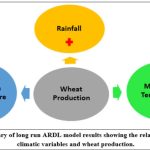Figure 4: Summary of long run ARDL model results showing the relationship between climatic variables and wheat production.Click here to view Figure

Table 6 presents the coefficients, standard errors, t-statistics, and probabilities for the variables LNRF, LNMXT, and LNMNT. The positive coefficient for LNRF indicates that, on average, a one percent increase in LNRF is associated with a 0.276 percent increase in wheat production. However, this effect is statistically insignificant, as reflected by the t-statistic of 0.685 and a p-value of 0.499. The small t-statistic suggests that the relationship lacks statistical significance. Overall, the results point to a positive correlation between rainfall and wheat output, higher rainfall tends to enhance production, whereas insufficient rainfall results in losses. This pattern is consistent with earlier research on wheat and rainfall, including studies.^21-24 The negative coefficient for LNMXT shows that, on average, a one percent increase in maximum temperature leads to a 0.678 percent decline in wheat production. The specific temperature thresholds that affect wheat yields may vary based on the wheat variety and the broader climatic conditions of the region. Elevated temperatures during sensitive growth stages can lower yields, reduce grain quality, and heighten susceptibility to pests and diseases. This highlights the significant role of maximum temperature in shaping wheat production.^25,26 identify maximum temperature as a key factor influencing wheat output, a finding supported by other studies such as.^27,28

The positive coefficient for LNMNT indicates that, on average, a one percent increase in minimum temperature corresponds to a 0.219 percent increase in wheat production. This suggests a positive relationship between minimum temperature and wheat output, underscoring its importance in wheat cultivation. Minimum temperature plays a crucial role at various stages of crop development. Favourable temperatures during critical phases such as germination and flowering can enhance yields, while moderate minimum temperatures generally support optimal growth.

Table 7: Shows  short run co-integration in ARDL Model

Variable	Coefficient	Std. Error	t-Statistic	Prob.
D(LNRF)	0.05	0.04	1.18	0.25
D(LNMXT)	0.83	0.30	2.79	0.01
D(LNMNT)	-0.12	0.12	-0.95	0.35
CointEq(-1)*	-0.14	0.06	-2.43	0.02

Source; Author’s Calculation Eview-10

Table 7 reports the coefficients, standard errors, t-statistics, and probabilities for the short-run Auto Regressive Distributed Lag (ARDL) model. The positive coefficient for LNRF shows that a one percent increase in LNRF is associated with a 0.05 percent increase in wheat production. However, the t-statistic of 1.18 and the p-value of 0.25 indicate that this relationship is not statistically significant at conventional levels (e.g., 0.05). This suggests that short-term fluctuations in LNRF may not have a reliable effect on wheat production.

The positive coefficient for LNMXT indicates that a one percent increase in maximum temperature corresponds to a notable 0.83 percent increase in wheat production. The t-statistic of 2.79 and the low p-value of 0.01 confirm the statistical significance of this relationship. Thus, in the short run, changes in LNMXT appear to exert a significant influence on wheat output.

The negative coefficient for LNMNT suggests that a one percent rise in minimum temperature results in a 0.12 percent decline in wheat production. However, the t-statistic of 0.95 and the p-value of 0.35 indicate that this relationship is not statistically significant, implying that short-run variations in LNMNT may not consistently affect wheat production. The Error Correction Term (ECT) is statistically significant and negative at 0.14, indicating an annual disequilibrium adjustment of 14 percent. This reflects a gradual correction toward long-run equilibrium over time.

Table 8: Model of Summary

R-squared	0.6741	Mean dependent var	0.009
Adjusted R-squared	0.6406	S.D. dependent var	0.069
S.E. of regression	0.0605	Akaike info criterion	-2.655
Sum squared resid	0.1026	Schwarz criterion	-2.471
Log likelihood	46.4731	Hannan-Quinn criter.	-2.594
Durbin-Watson stat	2.1081

Source: Author’s Calculation Eview-10

Table 8, the provided output is from a regression analysis, providing various statistics to evaluate the performance and goodness of fit of the model.  The R-squared value indicates the proportion of the variation in the dependent variable (DV) explained by the independent variables (IVs) in the model. In this case, approximately 67.41% of the variability in the DV is accounted for by the model. The Durbin-Watson statistic tests for the presence of autocorrelation in the residuals. A value close to 2 suggests no significant autocorrelation.

Table 9: Diagnostic Test

Diagnostic Test	F-statistic	Prob
Breusch-Godfrey Serial Correlation LM Test:	0.222	0.80
Heteroskedasticity Test: Breusch-Pagan-Godfrey	0.411	0.89
Histogram Normality Test	3.27	0.19

Source; Author’s Calculation Eview-10

Table 9 reports the results of three diagnostic tests commonly used in regression analysis to assess key aspects of model adequacy. The first test examines serial correlation in the residuals, evaluating whether residuals are correlated across different lags. The low F-statistic (0.222) and the relatively high p-value (0.80) indicate insufficient evidence to reject the null hypothesis of no serial correlation. This suggests that the residuals do not display a significant correlation pattern over time.

The second test assesses homoscedasticity, determining whether the variance of the residuals remains constant across observations. The F-statistic of 0.411 and the associated p-value of 0.89 suggest that there is no significant evidence against the null hypothesis of homoscedasticity. Thus, the residuals do not exhibit strong signs of variance instability. The third test evaluates the normality of the residuals, checking whether they follow a normal distribution. The chi-squared statistic yields a p-value of 0.19, which is not low enough to reject the null hypothesis at common significance levels (e.g., 0.05). Therefore, there is no strong evidence against the assumption of normality in the residuals.

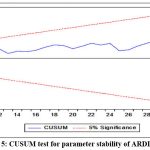Figure 5: CUSUM test for parameter stability of ARDL model.Click here to view Figure

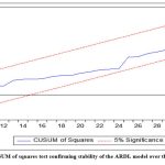Figure 6: CUSUM of squares test confirming stability of the ARDL model over the study period Click here to view Figure

Stability Model

The stability of the model is assessed through Figures 4 and 5, depicting the results of the CUSUM and CUSUM square tests. These tests are effective tools for detecting structural changes in time series data. The figures visually represent the cumulative sum and cumulative sum of squares, helping to identify any shifts or breaks in the stability of the model over time.

Conclusion and Policy Implication

This study applies trend analysis and the ARDL model to evaluate the impact of climate change on wheat production in Punjab. The results reveal a dynamic relationship between climate variables and wheat output over time. The positive coefficient for LNRF indicates that, on average, a one percent increase in LNRF is associated with a 0.276 percent increase in wheat production. However, this effect is statistically insignificant, as reflected by the t-statistic of 0.685 and a p-value of 0.499. The small t-statistic suggests that the relationship lacks statistical significance. Overall, the results point to a positive correlation between rainfall and wheat output, higher rainfall tends to enhance production, whereas insufficient rainfall results in losses. These findings offer important insights for policymakers in designing adaptive strategies, underscoring the need to promote climate-resilient farming practices and invest in water-use efficiency. Strengthening research and extension services is essential to equip farmers with climate-smart techniques. Moreover, comprehensive risk-management measures and insurance schemes are necessary to safeguard farmer’s livelihood.

Effective mitigation of climate change impacts will require coordinated efforts among government agencies, research institutions, and the agricultural community to ensure sustainable wheat production in Punjab. Nonetheless, the study faces certain limitations, including limited long-term data, difficulties in attributing changes solely to climate variables, and the complex interplay of multiple agricultural factors. These constraints may influence the study’s scope and its applicability across different regions within Punjab.

Acknowledgement

I am so grateful to each of the anonymous reviewers whose thoughtful feedback was more helpful than I can express. With all errors being mine, the paper is much improved for such generative comments.

Funding Sources

The author(s) received no financial support for the research, authorship, and/or publication of the article.

Conflict of Interest

The authors do not have any conflict of interest.

Data Availability Statement

Data Availability Statement: The data supporting the research findings are available in the RBI Handbook of Statistics on Indian States.

Ethics Statement

This section verifies that the research was carried out following ethical guidelines. It confirms that the study adhered to the necessary ethical standards and clarifies that there are no other related papers associated with this research.

Informed Consent Statement

This study did not involve human participants, and therefore, informed consent was not required.

Permission to reproduce material from other sources

Not Applicable

Author Contributions

Yasser Hussain: introduction, methodology and analysis

Aasima Nazir: the review of literature, conclusion and summary

References

1. Aggarwal PK, Kalra N, Chander S, Pathak H. Info Crop: A dynamic simulation model for the assessment of crop yields, losses due to pests, and environmental impact of agro-ecosystems in tropical environments. I. Model description. Agric Syst. 2000; 65(2):145-171.
2. Ansari S, Ansari SA, Khan A. Does agricultural credit mitigate the effect of climate change on sugarcane production? Evidence from Uttar Pradesh, India. Curr Agric Res J. 2023; 11(1).
   CrossRef
3. Ansari S, Ansari SA, Rehmat A. Determinants of instability in rice production: empirical evidence from Uttar Pradesh. J ANGRAU. 2022; 104.
4. Ansari S, Jadaun KK. Agriculture productivity and economic growth in India: an ARDL model. South Asian J Soc Stud Econ. 2022; 15(4):1-9.
   CrossRef
5. Ansari S, Rashid M, Alam W. Agriculture production and economic growth in India since 1991: an econometric analysis. Dogo Rangsang Res J. 2022; 12(3):144-146.
6. Amir M, Ansari S, Khan F, Rashid M. Do climate changes influence the food grain production in India: an ARDL model. Korea Rev Int Stud. 2023; 45(15):1-9.
7. Deressa TT, Hassan RM, Ringler C, Alemu T, Yesuf M. Determinants of farmers’ choice of adaptation methods to climate change in the Nile Basin of Ethiopia. Glob Environ Change. 2011; 21(2):764-770.
8. Intergovernmental Panel on Climate Change (IPCC). Climate Change 2014: Synthesis Report. Geneva, Switzerland: IPCC; 2014.
9. Kaur P, Aggarwal PK, Jain N, Pathak H. Climate change and wheat yields in Punjab, India: testing the value of spatial downscaling for adaptation decision-making. Agric Syst. 2018; 163:12-22.
10. Khan A, Ansari SA, Ansari S. Growth performance of major food-grain (wheat, rice and gram) in Uttar Pradesh: an economic analysis. Int J Curr Microbiol Appl Sci. 2023; 12(1):196-202.
    CrossRef
11. Khan A, Ansari SA, Ansari S, et al. Growth and trend in area, production, and yield of wheat crops in Uttar Pradesh: a Johansen co-integration approach. Asian J Agric Ext Econ Sociol. 2023; 41(2):74-82.
    CrossRef
12. Khan A, Ansari A, Khan MS, Ansari S. The impact of financial sector, renewable energy consumption, technological innovation, economic growth, industrialization, forest area and urbanization on carbon emission: new insight from India. Korea Rev Int Stud. 2024; 17(54).
13. Kaur B, Kamal V, Sidhu RS. Optimizing irrigation water use in Punjab agriculture: role of crop diversification and technology. Indian J Agric Econ. 2015; 70(3):307-318.
14. Kumar S, Kaur B. Impact of climate change on the productivity of rice and wheat crops in Punjab. Econ Polit Wkly. 2019; 54(46):38-44.
15. Lal M, Nozawa T, Emori S, et al. Future climate change: implications for Indian summer monsoon and its variability. Curr Sci. 2001; 81(9):1196-1207.
16. Lal M, Singh KK, Rathore LS, Srinivasan G, Saseendran SA. Vulnerability of rice and wheat yields in NW India to future changes in climate. Agric For Meteorol. 1998; 89(2):101-114.
    CrossRef
17. Lobell DB, Bänziger M, Magorokosho C, Vivek B. Nonlinear heat effects on African maize as evidenced by historical yield trials. Nat Clim Change. 2011; 1(1):42-45.
    CrossRef
18. Mahmood N, Ahmad B, Hassan S, Bakhsh K. Impact of temperature and precipitation on rice productivity in rice-wheat cropping system of Punjab province. J Anim Plant Sci. 2012; 22:993-997.
19. Meng Q, Qi Y, Du S, Cui Y, Luo Q. Impact of climate change on wheat yield in China from 1981 to 2015. Agric For Meteorol. 2018; 262:233-241.
20. Prasad R, Shivay YS. Agricultural changes in north-western India as influenced by green revolution and irrigation water availability. Int J Bioresour Stress Manag. 2022; 13(12):1355-1359.
    CrossRef
21. Reynolds MP, Quilligan E, Aggarwal PK, et al. An integrated approach to maintaining cereal productivity under climate change. Glob Food Sec. 2016; 8:9-18.
    CrossRef
22. Rashid M, Ansari S, Khan A, Amir M. The impact of FDI and export on economic growth in India: an empirical analysis. Asian J Econ Finance Manag. 2023:83-91.
23. Schlenker W, Roberts MJ. Nonlinear temperature effects indicate severe damages to U.S. crop yields under climate change. Proc Natl Acad Sci USA. 2009; 106(37):15594-15598.
    CrossRef
24. Singh RD, Kumar CP. Impact of climate change on groundwater resources. CC-RDS. Roorkee: National Institute of Hydrology; 2009.
25. Singh H. Impacts of Green Revolution on cropping pattern in Punjab, India. Natl Geogr J India. 2022; 68(1).
    CrossRef
26. Singh J, Yadav HS, Singh N. Crop diversification in Punjab agriculture: a temporal analysis. J Environ Sci Comput Sci Eng Technol. 2013; 2(2):200-205.
27. Sidhu RS, Kamal V, Lal U. Climate change impact and management strategies for sustainable water-energy-agriculture output in Punjab. Indian J Agric Econ. 2011; 66(3):328-339.
28. Vashisht BB, Mulla DJ, Jalota SK, Kaur S, Kaur H, Singh S. Productivity of rainfed wheat as affected by climate change scenario in north-eastern Punjab, India. Reg Environ Change. 2013; 13:989-998.
    CrossRef
29. Zhang H, Wang Q, Li L, Guo L, Chen X, Zeng H. Impacts of climate change on the yield of winter wheat at different growth stages in China. J Integr Agric. 2020; 19(5):1322-1332.