Validation of AquaCrop for Deficit Irrigation on Garlic (Allium sativum L.) for Semi-arid Conditions

Introduction

Like any other crop, garlic requires different amounts of irrigation depending on the area.  Garlic’s crop water needs are not uniformly distributed throughout the growing season; rather, they are mostly determined by the species, growth stages, soil characteristics, and climate.¹ Given that agriculture uses more than 70% of the world’s freshwater,¹⁰ managing limited water resources effectively in water-stressed areas,such as semi-arid areas, is significant challenge for irrigation water managers. As a result, sustainable and efficient agricultural water management is essential in these water-stressed areas. Therefore, water-saving irrigation techniques like deficit irrigation (DI) should be used as part of an on-farm plan for irrigation water management.²The AquaCrop model might be utilised to investigate crop’s reaction to different water application amounts, considering the constraints associated with garlic production in semi-arid conditions.⁴DI is the deliberate technique of irrigating crops below their crop water requirements in order to subject them to a particular degree of water stress.⁶ Farmers may experience a certain amount of production loss when implementing DI practices.  The subjective nature of soil moisture measurement is one of the main problems with this method.  In this sense, an overabundance of irrigation water may not only reduce productivity but also have additional detrimental effects, like nutrient leaching and groundwater rise.⁶ Modelling tools that assist management choices for effective water utilisation in agricultural production are needed in this scenario. A decision support tool for modelling and developing globally applicable strategies for effective AquaCrop management, the AquaCrop model has to be evaluated in many locations with varying soil conditions and crop-water productivity at the farm level.⁸However, a significant amount of water can be conserved, which could be utilised to expand and cultivate more land, thus improving food output.^9&10Agronomic methods, climate, and agricultural production. The implementation of effective water management strategies would ultimately result in a greater understanding of how to increase garlic yield.

Physiological mechanisms, crop traits, growth, yield, data extrapolation, and prediction are all aided by the models.⁸ Additionally, simulation models are mostly utilized as prediction tools to assist in making best decisions in the future.⁹  The recommendations for managing water resources that can be obtained when utilising crop simulation model to specific agricultural system problems may differ based on which element is prioritised over another.¹¹ In water-stressed areas, these crop models were very helpful in assessing and creating alternative methods for increasing crop output while using less irrigation water.¹¹ For instance, strict irrigation schedules could be required to maximise crop productivity and profitability.Models for crop simulation were created and used in agricultural water management.¹⁴ On the other hand, lowering drainage water loss and increasing WP might support a smaller water supply.  It becomes abundantly clear that all of the many system components that are directly related to irrigation techniques must be taken into account when optimising water resources.³ However, more intricate, multi-objective assessments that tackle conflicting goals, including increasing water efficiency, minimising environmental impact, and maximising yield, can be supported by crop simulation models.⁴

Rain-fed, deficiency, supplementary, and full irrigation circumstances are the four scenarios in which model replicates yield of numerous herbaceous crops.¹³ AquaCrop is simpler to use than other models and enables the simulation of crop performance using a variety of circumstances.  Additionally, it has a higher degree of precision and needs fewer input parameters. This study suggested a hierarchical structure intended to streamline the irrigation strategy optimisation process to overcome this complexity and achieve significant advancements.¹⁵ First, AquaCrop model was calibrated as well as validated by utilzing field data to guarantee precision and reliability of the model’s predictions.¹¹To investigate a wide range of irrigation possibilities, different irrigation scenarios were built on top of this base.  With this method, an empirical model based on second-order polynomial regressions between irrigation volumes and water-related factors might be developed.⁴In the semi-arid region of Maharashtra (India), the primary goal of the current research was to test and calibrate AquaCrop model for simulating garlic yield/growth and water-use characteristics under varying irrigation volumes and mulch materials.

Materials and Methods

Description of Study Area

During rabi season, a trial was conductedfrom 19 Dec. 2021 to 26 April. 2022 at Mahatma Phule Krishi Vidyapeeth, Rahuri, Maharashtra. It is 657 meters above mean sea level and is between latitudes 19°–48° N and 19°–57° N, longitudes 74°–32°E and 76°–19°.  The Rahuri region experiences modest temperature fluctuations and a mainly semi-arid climate.  The majority of the soil at the research site is heavy clay, which retains moisture well and has low permeability.  Long-term weather records show that the study area receives 450–550 mm of rainfall annually, with July and August seeing the highest amounts. This rainfall happens 70% of the time from mid-June to mid-September. Average minimum and maximum temperatures in Rahuri, Maharashtra, are 35°C (95°F) and 23°C (73°F) in March. The average annual temperature in Rahuri is 29°C (84°F). The research area’s restricted groundwater resource serves as the supply of irrigation water.

Material

Experiment has been laid out with 27 treatments with 3 replications. A drip irrigation system has been used to apply irrigation. Applying water directly to area close to roots helps prevent extensive percolation and leakage loss throughout the plot. The following pipe network was used in the drip irrigation system.

Filtration System

Sand Filter and Screen Filter

Pipe Network

Main line- 75mm

Submain-32mm

Lateral- Inline lateral

Spacing of dripper – 40 cm

Dripper Discharge- 4 Lph

Cultural Practices

Following site preparation, garlic seed was sown with a 20 cm x 15 cm crop spacing, yielding 533 plants per plot.  We utilized a block size of 48 × 49 m and an individual plot area of 16m², which is 4m×4m.  Every plot and replication was spaced 1.5 and 2 meters apart, respectively.  The goal of this separation is to reduce the amount of water that moves laterally between plots.  2 weeks after transplanting and 4 weeks before harvesting, 400 kg ha-1 of NPK (100:50:50) fertiliser was applied in two applications. The first application of weedicide (Oxyflurofen 23.5 and Quizalofop Ethyl 5%) was made 15 days after the garlic first appeared.  In order to manage weed development during the stages of crop growth, hand weeding was employed.  The field was also treated with fungicide (active ingredient: Azoxystrobin 23% SC, Amistar) and insecticide (active ingredient: carbosulfan 25% EC, Marshal) two and eight weeks after planting.  When available soil moisture dropped to 50%, the soil moisture depletion strategy was used to water as needed, beginning two weeks after planting.

Experimental design

Table 1 shows the field experiment’s randomised block design (RBD) setup, which included three replications and twenty-seven treatments with varying combinations of water stress at various growth stages.

Water stress

Garlic crop exposed water stress at every crop growth stage. The water stress is under as,

0 % water stress i.e. 100% water applied

30 % water stress i.e. 70% water applied

60 % water stress i.e. 40% water applied

Crop growth stages

The garlic crop was considered in three crop growth stages under and treatment combination presented in Table1.

Vegetative stage (VS) – 0-50 DAP

Bulb initiation stage (BI) – 50- 75 DAP

Bulb development stage (BD) – 75 to harvest

There were three replications and 27 treatment combinations in the randomised block design experiment.The treatment combination for vegetative stress, bulb initiation stage, and bulb development stage for no stress, 30% water stress, and 60% water stress is given below. The treatment T₁ was no water stress treatment in all growth stages; conversely, treatment T₂₇ is highest water stress treatment, i.e. 60% water stress was applied in entire growth period. In treatment T₂ to T₂₆ stress combination presented in Table 1.

Table 1: Treatments combination

1.	T1	VS -No stress (0.00S), BI-No stress (0.00S), BD-No stress (0.00S)
2.	T2	VS -No stress (0.00S), BI-No stress (0.00S), BD-Moderate stress (0.30S)
3.	T3	VS -No stress (0.00S), BI-No stress (0.00S), BD-High stress (0.60S)
4.	T4	VS -No stress (0.00S), BI-Moderate stress (0.30S), BD-No stress (0.00S)
5.	T5	VS -No stress (0.00S),  BI-Moderate stress (0.30S), BD- Moderate stress (0.30S)
6.	T6	VS -No stress (0.00S),  BI-Moderate stress (0.30S), BD- High stress (0.60S)
7.	T7	VS -No stress (0.00S),  BI-High stress (0.60S), BD-No stress (0.00S)
8.	T8	VS – No stress (0.00S), BI- High stress (0.60S), BD- Moderate stress (0.30S)
9.	T9	VS – No stress (0.00S), BI- High stress (0.60S), BD- High stress (0.60S)
10.	T10	VS -Moderate stress (0.30S), BI-No stress (0.00S), BD-No stress (0.00S)
11.	T11	VS -Moderate stress (0.30S), BI-No stress (0.00S), BD- Moderate stress (0.30S)
12.	T12	VS -Moderate stress (0.30S), BI-No stress (0.00S), BD- High stress (0.60S)
13.	T13	VS-Moderate stress (0.30S), BI- Moderate stress (0.30S), BD-No stress (0.00S)
14.	T14	VS-Moderate stress (0.30S), BI- Moderate stress (0.30S), BD- Moderate stress (0.30S)
15.	T15	VS-Moderate stress (0.30S), BI- Moderate stress (0.30S), BD- High stress (0.60S)
16.	T16	VS-Moderate stress (0.30S), BI- High stress (0.60S), BD-No stress (0.00S)
17.	T17	VS-Moderate stress (0.30S), BI- High stress (0.60S), BD- Moderate stress (0.30S)
18.	T18	VS-Moderate stress (0.30S), BI- High stress (0.60S), BD- High stress (0.60S)
19.	T19	VS-High stress (0.60S), BI-No stress (0.00S), BD-No stress (0.00S)
20.	T20	VS- High stress (0.60S), BI-No stress (0.00S), BD- Moderate stress (0.30S)
21.	T21	VS- High stress (0.60S), BI-No stress (0.00S), BD- High stress (0.60S)
22.	T22	VS- High stress (0.60S), BI- Moderate stress (0.30S), BD-No stress (0.00S)
23.	T23	VS- High stress (0.60S), BI- Moderate stress (0.30S), BD- Moderate stress (0.30S)
24.	T24	VS- High stress (0.60S), BI- Moderate stress (0.30S), BD- High stress (0.60S)
25.	T25	VS- High stress (0.60S), BI- High stress (0.60S), BD-No stress (0.00S)
26.	T26	VS- High stress (0.60S), BI- High stress (0.60S), BD- Moderate stress (0.30S)
27.	T27	VS- High stress (0.60S), BI- High stress (0.60S), BD- High stress (0.60S)

Data Collection

Farmland observations and measurements were used to gather primary field data.

Climatic Data

Daily climatic data involving maximum as well as minimum sunshine, temperature, relative humidity, rainfall, wind speed, evaporation have been collected from meteorological observatory of “Mahatma Phule Krishi Vidyapeeth, Rahuri”.¹⁴ Reference evapotranspiration has been calculated by utilising Penman-Monteith equation andmeteorological data as follows:

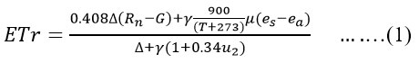
Where,

ETr = Reference evapotranspiration (mm day^-1)

R_n = Net radiation at crop surface (MJ m^-2 day^-1) is the difference among incoming and outgoing solar radiation.

G = Soil heat flux density (MJ m^-2 day^-1)is rate at which heat energy is transferred between Earth’s surface and underlying soil

T = Mean daily temperature at 2m height (^oC)

u₂= Wind speed at 2m height (m s^-1)

e_s= Saturation vapour pressure (kpa), pressure of a vapour when it’s in equilibrium with its liquid or solid phase at a given temperature. 

e_a= Actual vapour pressure (kpa), refers to partial pressure of water vapour in air, representing amount of water vapour present in a given volume of air.

(e_s – e_a)= Saturation vapour pressure deficit (kpa), Difference among saturation vapor pressure and actual vapor pressure

∆ = Slope of vapour pressure curve (kpa^oC^-1)

γ = Psychrometric constant (kpa^oC^-1)is a factor used in calculations involving partial pressure of water vapour in air, particularly in context of humidity and evaporation.

Evapotranspiration Water Productivity

Equation 3 was used to determine the evapotranspiration water productivity.⁵

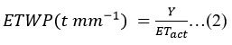
where Y isactual yield (tha-1), ETactisactual evapotranspiration (mmha-1), and ETWP is the evapotranspiration water productivity (tmm^-1).

Calibration and Validation of AquaCrop Model

Climate data, including daily maximum as well as minimum daily rainfall, air temperatures (T), daily atmospheric evaporative demand expressed as reference Eto (evapotranspiration) from Meteorological Services, and default mean annual carbon dioxide concentration for climatic file, were used to simulate AquaCrop model. After choosing the crop type, AquaCrophas been utilised to produce entire set of necessary crop parameters in order to create the crop file.  Three stages of growth—vegetative, bulb commencement, and bulb development—were taken into account.  Additionally, irrigation files were made for every experimental treatment. This allowed for the specification of the irrigation events’ timing and depth of application.  Type of soil (soil texture), soil depth, as well as a few other data were used to build the soil file.  For every treatment, crop yield and evapotranspiration water productivity were calculated, and the results were verified by contrasting them with the AquaCrop-modelled results.

Data Analysis

ANOVA(Analysis of variance) was utilised to statistically assess agronomic parameters that have been entered into a Microsoft Excel spreadsheet.  Statistical techniques, such as standard deviation and Nash-Sutcliffe model efficiency (E),^7,16 which were expressed using Equation (4), were then used to evaluate the model’s performance.

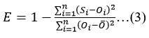
RMS Eexpressed as

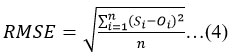
and the Index of Agreement (d),^12,13 also expressed as

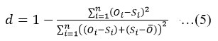
where n is number of observations, O ̅ is mean value, and  Oi andSi are observed and predicted data, correspondingly.

Results

Evapotranspiration Water Productivity

The actual evapotranspiration shown in Table 2 has been used to determine evapotranspiration water productivity.  Evapotranspiration water productivity of garlic various irrigation treatments ranged 0.025 to 0.023 t mm^-1. The highest irrigation water productivity 0.025 t ha^-1mm^-1was recorded in lowest water stress treatment T₁, T₂,T₃,T₄,T₅,T₁₁,T₁₂,T₁₇,T₂₁, and T₂₂, where as lowest 0.022 t ha^-1mm^-1 was recorded in high water stress treatment T₂₇. This suggests that when irrigation water regimes are reduced, evapotranspiration water productivity falls.

Table 2: Actual evapotranspiration water productivity (t mm^-1) influenced by different treatments

Sr. No.	Treatments	Yield (t ha-1)	Actual ETc (mm)	ETWP (t ha-1mm-1)
T1	VS (0.00S), BI (0.00S), BD (0.00S)	7.80	318.25	0.025
T2	VS (0.00S), BI (0.00S), BD (0.30S)	7.40	295.55	0.025
T3	VS (0.00S), BI (0.00S), BD (0.60S)	7.20	291.58	0.025
T4	VS (0.00S), BI (0.30S), BD (0.00S)	7.03	279.78	0.025
T5	VS (0.00S),  BI (0.30S), BD (0.30S)	6.80	265.45	0.025
T6	VS (0.00S),  BI (0.30S), BD (0.60S)	6.40	274.05	0.023
T7	VS (0.00S),  BI(0.60S), BD (0.00S)	6.67	285.53	0.023
T8	VS (0.00S), BI (0.60S), BD (0.30S)	6.43	273.67	0.023
T9	VS (0.00S), BI (0.60S), BD (0.60S)	6.32	265.23	0.024
T10	VS (0.30S), BI (0.00S), BD (0.00S)	7.18	295.15	0.024
T11	VS (0.30S), BI (0.00S), BD (0.30S)	7.01	283.73	0.025
T12	VS (0.30S), BI (0.00S), BD (0.60S)	6.80	277.22	0.025
T13	VS (0.30S), BI (0.30S), BD (0.00S)	6.90	286.62	0.024
T14	VS (0.30S), BI (0.30S), BD (0.30S)	6.60	278.21	0.024
T15	VS (0.30S), BI (0.30S), BD (0.60S)	6.30	277.29	0.023
T16	VS (0.30S), BI (0.60S), BD (0.00S)	6.71	276.75	0.024
T17	VS (0.30S), BI (0.60S), BD (0.30S)	6.54	265.78	0.025
T18	VS (0.30S), BI (0.60S), BD (0.60S)	6.23	257.80	0.024
T19	VS (0.60S), BI (0.00S), BD (0.00S)	7.15	287.69	0.025
T20	VS (0.60S), BI (0.00S), BD (0.30S)	6.85	279.79	0.024
T21	VS (0.60S), BI (0.00S), BD (0.60S)	6.90	270.01	0.025
T22	VS (0.60S), BI (0.30S), BD (0.00S)	6.80	269.78	0.025
T23	VS (0.60S), BI (0.30S), BD (0.30S)	6.50	273.24	0.024
T24	VS (0.60S), BI (0.30S), BD (0.60S)	6.20	258.72	0.024
T25	VS (0.60S), BI (0.60S), BD (0.00S)	5.90	242.56	0.024
T26	VS (0.60S), BI (0.60S), BD (0.30S)	5.50	236.94	0.023
T27	VS (0.60S), BI (0.60S), BD (0.60S)	5.10	233.85	0.022

Calibration and Simulation of AquaCrop Model

Ability of calibrated AquaCrop model to forecast crop production and evapotranspiration water productivity (ETWP) was evaluated. As shown in Table 3, the measured results from the experiment were compared with the simulated garlic production and evapotranspiration water productivity of various irrigation treatments. For irrigation treatments with no water stress and low water stress, like T₁ to T₉, crop yield was overestimated; for irrigation treatments with medium and severe water stress, like T₁₀ to T₂₇, crop yield was underestimated. The maximum observed and simulated yield was obtained in treatment T₁ were 7.80 t ha^-1 8.08 t ha^-1correspondingly, conversely lowest observed and simulated yield was obtained in treatment T₂₇ were 5.10 and 4.69 t ha^-1,correspondingly.Differenceamong simulated and actual crop yields ranged from 3.47 percent to -18.26%. In both situations, the irrigation treatment with no water stress recorded the highest, whereas the one with significant water stress recorded the lowest.  However, the AquaCrop model’s simulation of evapotranspiration water productivity was understated.  Table 4 shows the range of deviations from this.

Table 3: Observed and simulated ET during calibration of AquaCrop model

Treatment	Observed yield (t ha-1)	Simulated yield (t ha-1)	Deviation (%)	Actual ET (mm)	Simulated ET (mm)	Deviation (%)
T1	7.80	8.08	3.47	318.25	288.5	-10.31
T2	7.40	7.74	4.39	295.55	363.5	18.69
T3	7.20	7.57	4.89	291.58	281.8	-3.47
T4	7.03	7.46	5.76	279.78	300.6	6.93
T5	6.80	7.37	7.73	265.45	358.7	26.00
T6	6.40	7.30	12.33	274.05	349.1	21.50
T7	6.67	7.15	6.71	285.53	339	15.77
T8	6.43	6.95	7.48	273.67	337.5	18.91
T9	6.17	6.55	5.80	265.23	258.3	-2.68
T10	7.18	7.15	-0.42	295.15	346.7	14.87
T11	7.01	6.94	-1.01	283.73	289.0	1.82
T12	6.80	6.71	-1.34	277.22	283.8	2.32
T13	6.60	6.56	-0.61	286.62	281.1	-1.96
T14	6.30	6.32	0.32	278.21	277.0	-0.44
T15	6.90	6.26	-10.22	277.29	274.9	-0.87
T16	6.71	5.99	-12.02	276.75	315.1	12.17
T17	6.54	5.53	-18.26	265.78	307.8	13.65
T18	6.23	5.37	-16.01	257.80	293.7	12.22
T19	7.15	6.90	-3.62	287.69	338.6	15.04
T20	6.85	6.39	-7.20	279.79	328.1	14.72
T21	6.90	6.33	-9.00	270.01	278.3	2.98
T22	6.80	5.82	-16.84	269.78	263.9	-2.23
T23	6.50	5.68	-14.44	273.24	260.6	-4.85
T24	6.20	5.42	-14.39	258.72	255.0	-1.46
T25	5.90	5.25	-12.38	242.56	245.8	1.32
T26	5.50	5.00	-10.00	236.94	240.7	1.56
T27	5.10	4.69	-8.74	233.85	239.6	2.40

Table 4:  Simulated evapotranspiration water productivity

Treatment	Simulated Yield (t ha-1)	Simulated ET (mm)	ETwp (t ha-1 mm-1)
T1	8.08	288.5	0.028
T2	7.74	363.5	0.021
T3	7.57	281.8	0.027
T4	7.46	300.6	0.025
T5	7.37	358.7	0.021
T6	7.30	349.1	0.021
T7	7.15	339	0.021
T8	6.95	337.5	0.021
T9	6.55	258.3	0.025
T10	7.15	346.7	0.021
T11	6.94	289.0	0.024
T12	6.71	283.8	0.024
T13	6.56	281.1	0.023
T14	6.32	277.0	0.023
T15	6.26	274.9	0.023
T16	5.99	315.1	0.019
T17	5.53	307.8	0.018
T18	5.37	293.7	0.018
T19	6.90	338.6	0.020
T20	6.39	328.1	0.019
T21	6.33	278.3	0.023
T22	5.82	263.9	0.022
T23	5.68	260.6	0.022
T24	5.42	255.0	0.021
T25	5.25	245.8	0.021
T26	5.00	240.7	0.021
T27	4.69	239.6	0.020

The variations noted in this investigation are also consistent with Muhammad and Hussain’s (2012) findings that the model’s ability to predict yield and water productivity was good.  Crop structure and phenology, rather than climate, soil, and water supply conditions, may be the cause of the results’ variations. Simulated evapotranspiration water productivity is ratio of simulated yield to simulated evapotranspiration. Maximum simulated evapotranspiration recorded in no water stress treatment (T₁) is 0.028 t ha^-1 mm^-1, and lowest in high water stress treatment (T₂₇) is 0.020 t ha^-1 mm^-1. Water application differences were the cause of the variation in evapotranspiration water productivity.

Validation of AquaCrop model

Table 5 displays the statistical tools used to validate the AquaCrop model using the Nash-Sutcliffe efficiency (E), RMSE, and index of agreement (d).

Table 5: Validation of AquaCropmodel

Parameter	Efficiency Criteria
	Nash Coefficient	RMSE	Index of Agreement
Yield (t ha-1)	-0.035	0.57	0.83
Evapotranspiration Water Productivity (kg m-3)	-3.65	38.44	0.483

According to the data, the evapotranspiration water productivity was -3.65, and the yield Nash-Sutcliffe efficiency (E) was -0.035.According to Nash-Sutcliffe efficiency,the model efficiency is very less for yield, and evapotranspiration water productivity indicates that model is not perfect fit for garlic in semi-aridconditions.Yield and evapotranspiration water productivity had corresponding RMSEs of 0.57 and 38.44.Positive value of RMSE indicates that model is not perfect fit for garlic under semi-arid conditions. Additionally, the yield and evapotranspiration water productivity indices of agreement were 0.83 and 0.483, respectively.The index of agreement for yield 0.83,indicating good fit of model for yield and index of agreement 0.483 for evapotranspiration water productivity is 0.483, indicating that fair fit of model. 

Discussion

In this research, a novel analytical approach for identifying most effective irrigation techniques depend on seasonal water supply quantities is provided.The agricultural system’s economic, environmental, and productive elements were all taken into account separately in this method before being combined into a single multi-aggregated index. The Nash coefficient, RMSE, and Index of Agreement comprised the framework’s structure.  The results of statistical indices like E, RMSE, and d show that the framework’s base was resilient due to careful calibration and validation.  To build the rest of the framework, AquaCrop’s parameterization principally sought to mimic water use and the end marketable yield (with a good alignment among observed and simulated data).  As a result, AquaCrop’s accuracy in reproducing crop yield and water consumption was evaluated, guaranteeing framework’s applicability for assessing economic and productive aspects of processing tomato cropping system as well as its environmental sustainability under various irrigation scenarios.⁴

Conclusion

Garlic’s crop production and evapotranspiration water productivity might be replicated using the AquaCrop model. All of the factors taken into consideration in the study were satisfactorily simulated by the AquaCrop model, according to validation using the E(Nash-Sutcliffe efficiency), RMSE, d(index of agreement).  However, rather than climate, soil, and water supply conditions, the variations in outcomes can be caused by elements like crop structure and phenology.  Together with cereals and cash crops, belowground stems and bulb-like crops should be taken into account for the water productivity model used in global agriculture to improve performance and produce more accurate findings.

Acknowledgment

We would like to express our sincere gratitude to MPKV, Rahuri, for their invaluable support in facilitating the completion of our research. We extend our appreciation to the dedicated scientists who generously provided us with the opportunity to conduct this research, thereby contributing to the advancement of knowledge in our field. Furthermore, we would like to acknowledge the Chatrapati Shahu Maharaj National Research Fellowship (SARTHI) based in Pune for their instrumental support in successfully executing our research endeavors. Their assistance has been instrumental in achieving our research goals, and we are truly grateful for their contribution.

Funding Sources

The grant number for funding as given as Go. No./Sarthi/Scholarship/CSMNRF-2021/2021-22/896.

Conflict of Interest

The authors do not have any conflict of interest

Data Availability Statement

The authors have permission to share data

Ethics Statement

This research did not involve human participants, animal subjects, or any material that requires ethical approval.

Informed Consent Statement

The sign informed consent statement is obtained.

Permission to reproduce material from other sources

Not Applicable

Author Contributions

Rahul Ashok Pachore: Writing – review and editing, Writing – original draft, Conceptualization.

Sachin Dingre: Writing – review and editing, Writing – original draft, Software, Methodology, Formal analysis, Data curation.

Mahanand Mane – review & editing, Methodology, Data curation.

Mahesh Patil: Writing – review & editing, Methodology, Data curation.

References

1. Askaraliev B., Musabaeva K., Koshmatov B., Omurzakov K., Dzhakshylykova Z. Development of modern irrigation systems for improving efficiency, reducing water consumption and increasing yields. Machinery & Energetics2024;15(3):47-59. doi: 10.31548/machinery/3.2024.47.
   CrossRef
2. Chukalla A.D., Krol M. S.,HoekstraA. Y. Green and blue water footprint reduction in irrigated agriculture: Effect of irrigation techniques, irrigation strategies and mulching. Hydrol. Earth Syst. Sci., 2015;19(12): 4877-4891.
   CrossRef
3. Corcoles J., DominguezA.,MorenoM., OrtegaJ.,De Juan J. A non-destructive method for estimating onion leaf area. Irish J. Agri. and Food Research. 2015;54(1): 17-30.
   CrossRef
4. Garofalo P., RiccardiM., Di Tommasi P., Tedeschi A., Rinaldi M.,  De Lorenzi F.AquaCrop model to optimise water supply for a sustainable processing tomato cultivation in the Mediterranean area: A multi-objective approach. Agril. Systems 2025; 223:104198.
   CrossRef
5. Molden, D.Accounting for Water Use the Productivity. System Wide Initiave for Water Management (SWIM) Institute1997, Colombo.
6. MuhammadN., Hussain A. Modelling the response of onion crop to deficit irrigation. Journal of Agricultural Technology.2012; 8(1): 393-402.
7. J.E. Nash, and J.V. Sutcliffe,River flow forecasting through conceptual models, part I — A discussion of principles, Journal of Hydrology1970;10(3):282-290
   CrossRef
8. RauffK.O.,Bello R.A review of crop growth simulation models as tools for agricultural meteorology. Agril. Sciences,2015;6(9): 1098-1105.
   CrossRef
9. Shanono N.J., NasidiN.M.,ZakariM.D.,BelloM.M.Assessment of field channels performance at Watariirrigation project, Kano, Nigeria. 1^st International Conference on Dryland, Centre for Dryland Agriculture, Bayero University Kano, Nigeria. 8-12 December, 2014;144-150.
10. ShanonoN.J.,NdirituJ. A conceptual framework for assessing the impact of human behaviour on water resource systems’ performance. Algerian J. Engi.&Tech.2020;3: 9-16. https://doi.org/http://dx.doi.org/10.5281/zenodo.3903787.
11. Toumi J., Er-Raki S., EzzaharJ.,KhabbaS.,JarlanL.,Chehbouni A. Performance assessment of AquaCrop model for estimating evapotranspiration, soil water content and grain yield of winter wheat in Tensift Al Haouz (Morocco): Application to irrigation management. Agri. Water Management. 2016; 163: 219-235.
    CrossRef
12. Willmott C. J. On the validation of models. Physical Geography 1981; 2: 184-194. http://doi.org10.1080/02723646.1981.10642213
    CrossRef
13. Willmott C. J. Some comments on the evaluation of model performance. Bulletin of the American Meteorological Society 1982; 63: 1309-1313. https://doi.org/10.1175/1520-0477(1982)063<1309:SCOTEO>2.0.CO;2
    CrossRef
14. www.mpkv.ac.in, climatic data, 2021-22 and 2022-23
15. ZakariM. D., Audu I., Shanono N.J., MainaM.M., AbubakarM.S.,MohammedD. Sensitivity analysis of crop water requirement simulation model (CROPWAT (8.0) at Kano River Irrigation Project, Kano, Nigeria. Proceedings for International Interdisciplinary Conference on Global Initiatives for Integrated Development (IICGIID) ChukwuemkaOdumegwu University, Igbariam Campus, Nigeria), 2015; 502–510.
16. Zeybek M. Nash-Sutcliffe efficiency approach for quality improvement. J. Applied Math.&Computation. 2018;2(11): 496-503.
    CrossRef