Modeling and Estimation of Reference Evapotranspiration using Machine Learning Algorithms: A Comparative Performance Analysis

Introduction 

According to NITI Aayog’s 2019 Composite Water Management Index report, the majority of groundwater (more than 60%) in India is utilized for irrigation. Because there aren’t enough suitable water management policies and technologies, conventional irrigation methods are applied in the various parts of the country without any quantification of crop-water requirements. As per the report, wheat and rice are the two main crops grown in India. Approximately seventy-four percentage of the area cultivated with wheat and sixty-five percentage of the area cultivated with rice faces severe water scarcity issues. In agriculture sector, efficient water saving techniques are required and quantification of crop-water requirements using the evapotranspiration method can be extremely important in this context. It combines the transpiration of plants and evaporation from groundwater supplies. Crop evapotranspiration (ETc) is calculated using ETo, a climatic parameter that solely depends on other climatic variables like wind speed, humidity, temperature, solar radiation, and sunshine hours. Allen RG et al. (1998)¹ elaborated The Food and Agriculture Organization of the United Nation’s FAO-PM56, a well-known empirical approach that requires many weather-related variables and constants. Numerous empirical models have been proposed by writers in the literature to estimate ETo. Hargreaves et al. introduced the idea of temperature-based ETo estimation, which yields outcomes more in line with FAO-PM56. Many weather observation stations use sensors and powerful computers to generate and record large amounts of meteorological data every day. This has motivated us to investigate a variety of machine learning algorithms in an effort to forecast ETo with accuracy. A new field called artificial intelligence promises to revolutionize agriculture by giving software intelligence. An artificial intelligence-based strategy helps measure irrigation water consumption and increase crop yields. One type of artificial intelligence tool is machine learning algorithms, which can process large amounts of data and reliably extract meaningful patterns.  It can be an alternative solution instead of using empirical methods that require complex computation work. Numerous authors have used machine learning and soft computing techniques since the turn of the century and discovered that they may be effective means of estimating ETo. In this section, a few techniques have been examined and discussed.

Khosravi K et al. (2019)² explained the capacity of a number of machine learning models and soft computing methods, including M5P, RF, RT, REPT, and KStar, as well as four adaptive neuro-fuzzy inference systems are applied and assessed to estimate ETo, Kisi O (2007)³ used Levenberg–Marquardt based  feed forward artificial neural network, Gocić M et al. (2015)⁴ applied support vector machine–wavelet, artificial neural network, genetic programming, and support vector machine–firefly algorithm, Feng Y  et al. (2016)⁵ explained wavelet neural network models, back-propagation neural networks optimized by genetic algorithms, and extreme learning machine, Sanikhani H  et al. (2019)⁶ used artificial intelligence techniques such as GRNN, MLP, RBNN, GEP, ANFIS-GP and ANFIS-SC, Feng Y et al. (2017)⁷ tested random forest and generalized regression neural network models, Fan J et al. (2018)⁸ applied tree-based ensemble algorithms, namely random forest, M5Tree, gradient boosting decision tree, and extreme gradient boosting models, Yamaç SS et al. (2019)⁹ evaluated k-nearest neighbor, artificial neural network, and adaptive boosting, Tabari H et el. (2013)¹⁰ demonstrated adaptive neuro-fuzzy inference system and support vector machines models, Valipour M. et al. (2017)¹¹ applied genetic algorithm and gene expression programming models, Granata F. (2019)¹² suggested M5P regression tree, bagging, random forest, and support vector regression, Abyaneh HZ  et al. (2011)¹³ used Artificial intelligence techniques included artificial neural network and adaptive neuro-fuzzy inference system, Aghajanloo MB (2013)¹⁴ tested artificial neural network, neural network–genetic algorithm, and multivariate nonlinear regression methods, Feng Y et al. (2017) ¹⁵ shown extreme learning machine and generalized regression neural network models, Wen X  et al. (2015)¹⁶ applied the support vector machine, Nema MK  et al. (2017)¹⁷ artificial neural network model with Levenberg–Marquardt training algorithm with a single hidden layer having nine neurons to quantified ETo of various regions across the world, Saggi MK  et al. (2019¹⁸ proposed H2O model framework to estimate ETo Hoshiarpur and Patiala district, Mehta R  et al. (2015)¹⁹ estimated the ETc of wheat and maize for various places of Gujarat.

This study investigates and compares the skills of three regression based supervised learning algorithms namely decision tree (dtr), and random forest (rfr), and k-nearest-neighbors (knnr) models for estimation of ETo. Many developing and underdeveloped countries lack the resources necessary to obtain the high-accuracy and reliable meteorological data. This encourages us to look into how well the model performs in different combinations of meteorological parameters, limited to what is necessary. Based on groups are created due to the significant relationship between meteorological parameters and ETo. Therefore, twelve different models are evaluated and contrasted here and aims to identify the better models to forecast ETo.

Materials and Methods

Datasets

This study’s daily meteorological data, which spans the years 2000–2021, was obtained from IMD, Pune. There are 8036 samples in it. New Delhi experiences a wide range of climates, from humid-subtropical to semi-arid, with significant variations in summer and winter temperatures (from -2.2⁰C to 49.2⁰C).  New Delhi, which lies in the northern part of the nation between the latitudes of 28°-24′-17″ and 28°-53′-00″ North and the longitudes of 76°-50′-24″ and 77°-20′-37″ East, with elevation of 217 meters. The data set consist with the daily temp_min (minimum temperature) and temp_max  (maximum temperature) in ⁰C, R_h (humidity) in percentage, u (wind speed) in m/s, and R_s (solar radiation) in MJ/m²/day. An explanation of New Delhi’s meteorological data statistically is appears in  Table 1. Table 2 displays the correlation coefficients between the meteorological data and the observed ETo by FAO-PM565 and visualize with the help of heat map in Fig. 1. Fig. 2 displays the weekly variation in the ETo of New Delhi. 

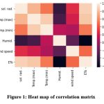Figure 1: Heat map of correlation matrix                  Click here to view Figure

Figure 2: Weekly variation in ETo of  New Delhi Click here to view Figure

Table 1: An explanation of New Delhi’s meteorological data statistically.

Parameters	Dataset	Maximum	Minimum	Mean	Standard Deviation
Temp_max (oC)	Training	48.79	12.55	33.0	7.06
	Test	48.05	14.33	32.79	7.09
Temp_min (oC)	Training	34.6	-1.36	19.18	8.10
	Test	34.30	-0.27	18.98	8.14
Rh(%)	Training	95.12	4.19	45.54	21.09
	Test	93.62	5.75	45.62	21.37
U (m/s)	Training	6.42	0.47	2.20	0.83
	Test	6.14	0.59	2.22	0.85
Rs(MJ/m2/day)	Training	30.02	1.47	17.59	5.41
	Test	28.54	1.98	17.32	5.54
ETo(mm/day)	Training	18.74	0.694	7.49	3.21
	Test	19.16	1.00	7.39	3.28

table 2: Matrix of correlation between New Delhi’s meteorological data and observed ETo

	New Delhi
	temp_max	temp_min	Rh	U	Rs	ETo
temp_max	1
temp_min	0.86	1
Rh	-0.33	0.12	1
U	0.21	0.07	-0.24	1
Rs	0.77	0.53	-0.40	0.28	1
ETo	0.84	0.53	-0.64	0.48	0.88	1

 FAO PM56 Equation

The FAO recommends the FAO-56 Penman-Monteith equation [1]. The well-known empirical technique for predicting ETo is displayed below:

where reference-evapotranspiration (mm/day) is represented by ETo. Net radiation is indicated by R_n (MJ m^-2 day^-1), The symbols G represent soil-heat flux (MJ m^-2 day^-1), γ the psychometric constant (kPa^oC^-1), T the mean temperature (^oC), and u₂ the wind speed at a height of 2 meters (m/s). Slope vapour pressure curve (kPa^oC^-1) is indicated by Δ, saturation vapour pressure (kPa) is indicated by e_s, and actual vapour pressure (kPa) is indicated by e_a.

K-nearest neighbor regression 

K-nearest-neighbors is one of the easiest, most effective, and non-parametric machine learning algorithms available. It comes under the category of a lazy classifier. Wang X  et al. (2018)²⁰  outlined the crisp knn algorithm’s concept that assigned unlabelled objects into appropriate classes according to k numbers of nearest neighbors. There are various approaches to finding the nearest neighbors. Euclidean Distance is one of them and the most popular distance metric approach and it is given in Eq. no. 2.   Apart from having the capability of classification of the knn algorithm, it is also able to solve regression problems. The k-nearest-neighbors regression (knnr) algorithm can estimates the value of a target variable (ETo). The ETo of test samples can be estimated using this method by utilizing k-nearest neighbours The closeness is decided by measuring the distance between the test sample and the k training samples. By averaging the ETo of nearly k training samples, the ETo of the test sample is inferred. Because of its simplicity, researchers are drawn to it to gain insight from datasets in a variety of fields. Various modified versions have been suggested to enhance the speed and accuracy of k-nearest-neighbors. The concept of fuzzy k-nearest-neighbors was also suggested to enhance the accuracy. In this investigation, the optimal value of the hyper-parameter number of neighbors (k-neighbors) is estimated in the k-fold cross validation which is further used during the training-testing period to achieve excellent performance.

Where

d is the distance and _Xk and _Yk are N- dim esion data point s

Decision tree regression 

A decision tree model with continuous target variables is called a decision tree regression algorithm (dtr). It is used to estimate the accurate value of target variables. Sutton CD. (2005)²¹ provided the procedure to create decision tree regression was given, where each node is recursively split into binary nodes in a top-down manner using the Greedy principle. Split is done at each node by locally minimizing the variance through mean squared error. Partitions are done at a particular point or mean of two adjacent points that have the least squared error. Various hyper-parameters can be assigned to manage The decision tree’s structure such as criteria to manage the quality of split, utmost depth of the tree, least samples at the leaf node, etc. In this investigation, the optimal value of hyper-parameter minimum samples at a leaf node (samples leaf) is estimated in the 5-fold cross validation which is used during the training-testing period to achieve excellent performance. Mean squared error has been opted for splitting criteria in the decision tree regression algorithm. Decision Tree may suffer from overfitting problems that are removed by either pre-pruning or post pruning. Random Forest is a kind of ensemble machine learning method that may play a vital part to eliminate overfitting problems.

Random forest regression

Breiman L (2001) ²² presented random forest regression (rfr) algorithm as  reliable tool without overfitting issues for predicting the desired value. This ensemble machine learning technique combines the results of several decision trees to estimate the target value based on majority voting, and it is applied to regression and classification problems. In the random forest regression algorithm, multiple decision trees are created iteratively on randomly selected training samples and features with replacement. Greater numbers of trees in random forest regression increase the accuracy. In this investigation, the forest’s decision trees’ (estimators’) ideal value is estimated in the k-fold cross validation, which is further used during the training-testing period to achieve excellent performance. Mean squared error has been opted for splitting criteria. Other hyper-parameters like utmost tree depth, least number of samples needed to split the node, maximum number of samples looking for the best split may have an impact on the random forest regression algorithm’s performance.

Model development

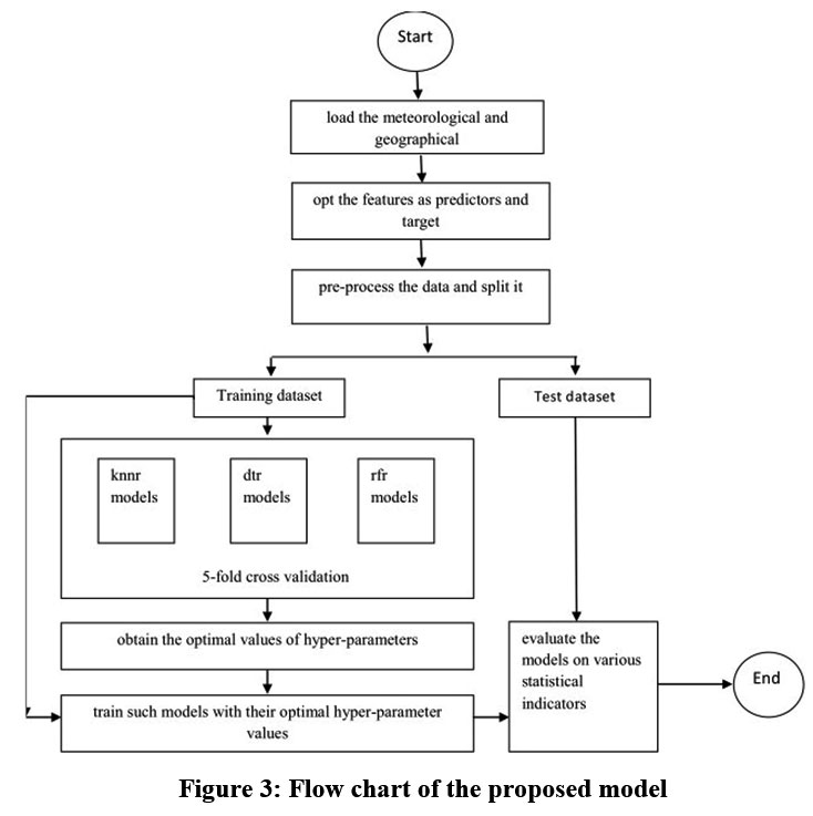Figure 3: Flow chart of the proposed model Click here to view Figure

To simulate the ETo, a flowchart of proposed models is presented in Fig. 3 and summarized in Algorithm_knnr.

Algorithm_knnr

Input: Meteorological and geographical data of New Delhi city.

Output: Simulated value of ETo.

Load the data set into memory.

Designate temp_min, temp._max, R_s, u and R_h as predictor and observed ETo (FAO-PM56) as response variable.

Fill the missing values and scaling the data (pre-processing).

Randomly split the dataset into training (80%) and test (20%) data.

Initialize hyper-parameter k-neighbors = 2.

Repeat step 7 to 9 until k-neighbors > 15.

Repeat step 8 for each combinations of predictors.

Perform 5-Fold cross validation (train knnr on each 4-Folds and validate it on remaining 1-Fold) and record the performance.

k-neighbors++.

Select optimal value of k-neighbors based on higher mean performance.

Estimate ETo by knnr on test data along with optimal value of k-neighbors.

Evaluate the performance of knnr on various statistical indicators (SI_i)

Similar steps are taken by Algorithm_rfr and Algorithm_dtr for varying hyper-parameter estimators (10 to 100) and sample-leaf (2 to 6), respectively.

The suggested model consists of several steps, such as gathering data, preprocessing it, determining the ideal hyper-parameter value, training the model, and assessing its effectiveness. The detail description of such steps are given below-

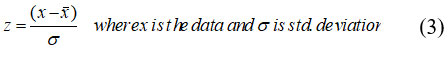
Initially, data is loaded into memory. Features in supervised machine learning algorithms need to be categorized and assigned to target and predictor features. In this study, performance of knnr, dtr and rfr models are compared on four combinations of meteorological parameters. In the combination-1, temp_min and temp._max are defined as predictor features. In the combination-2, temp_min, temp._max and R_s are defined as predictor features. In the combination-3, temp_min, temp._max, R_s and u are defined as predictor features. Similarly in the combination-4, temp_min, temp._max, R_s, u and R_h are defined as predictor features. ET_o calculated by the FAO-PM56 equation is defined as a target feature in all combinations.  Preprocessing of available data is a good practice in pattern recognition to obtain high skills of the models. In the present study the predictors are normalized with z-score normalization equation which is shown below

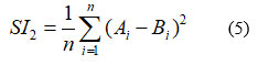
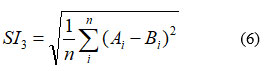
The observations from weather stations are randomly divided into two subsets: The model is trained using 80% of the data, and it is tested using the remaining 20%. Tuning of the hyper-parameters is carried out on the knnr, dtr, and rfr models along with four different combinations of input parameters to obtain the optimal value of it to achieve the high performance of such models. Three hyper-parameters are taken into consideration in this study: the number of neighbors (k-neighbour) in the knnr case, the minimum samples at a leaf node (samples leaf) in the dtr case, and the number of trees (estimators) in the rfr model case. On training datasets, five-fold cross validation is used to determine the ideal hyper-parameter value. Finally, the knnr, dtr, and rfr models with their optimal hyper-parameter are trained using 80% training datasets and tested with the remaining 20% datasets. The models’ performance is assessed using five statistical indicators (SI), including Mean absolute error(SI₁), Mean square error (SI₂), Root mean square error (SI₃), r/Pearson correlation coefficient (SI₄), r²/coefficient of determination or R-square (SI₅).

Performance evaluation indicators

Using the following statistical indicators equations, the performance of the knnr, dtr, and rfr models have been assessed in the current study:

SI₁–

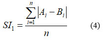
Where A_i = predicted ETo . B_i= observed ETo

 SI₂ –

 SI₃ –

SI₄–

SI₅–

Result And Discussion

Table 3: Residual description of models for New Delhi.

	knnr1	knnr2	knnr3	knnr4	dtr1	dtr2	dtr3	dtr4	rfr1	rfr2	rfr3	rff4
Mean	1.43e-15	4.97e-16	9.94e-16	5.48e-17	-1.50e-16	-4.82e-16	-1.01e-15	-1.21e-15	3.47e-16	-7.11e-16	1.28e-15	1.15e-15
Std.	1.16	0.81	0.46	0.16	1.28	0.93	0.61	0.38	1.22	0.83	0.45	0.18
Min	-4.33	-4.08	-3.20	-0.93	-4.09	-4.41	-2.80	-1.92	-4.54	-4.26	-2.80	-1.24
25%	-0.69	-0.37	-0.24	-0.09	-0.78	-0.46	-0.32	-0.21	-0.73	-0.39	-0.25	-0.09
50%	-0.06	-0.02	0.0007	-0.004	-0.04	-0.04	-0.0002	0.007	-0.06	-0.01	0.01	0.01
75%	0.06	0.03	0.02	0.08	0.07	0.04	0.03	0.02	0.06	0.03	0.02	0.01
max	5.33	4.06	2.11	1.20	6.03	4.72	2.29	1.44	5.46	4.16	2.02	0.08

Table 4: Performance comparison of models for  New Delhi

Statistical Indicators	knnr1	knnr2	knnr3	knnr4	dtr1	dtr2	dtr3	dtr4	rfr1	rfr2	rfr3	rff4
SI1	0.9474	0.599	0.378	0.1567	1.0366	0.6755	0.4678	0.3023	0.9834	0.611	0.375	0.1724
SI2	1.566	0.7145	0.2498	0.0429	1.8465	0.914	0.3937	0.1612	1.6949	0.74	0.2364	0.0489
SI3	1.2515	0.8453	0.4998	0.2071	1.3589	0.956	0.6275	0.4015	1.3019	0.8602	0.4863	0.2211
SI4	0.9247	0.9667	0.9891	0.9986	0.9117	0.9575	0.9817	0.9928	0.9186	0.9656	0.9895	0.9983
SI5	0.855	0.9344	0.9783	0.9972	0.8312	0.9169	0.9637	0.9856	0.8438	0.9324	0.9791	0.9965

 As was previously mentioned, meteorological data is split at random into training and test datasets. To find the ideal hyper-parameter value, the training dataset is subjected to five-fold cross-validation. The performance of the knnr, dtr, and rfr models is evaluated in this investigation on two distinct levels. During the 5-fold cross validation process, it is measured at the first level to find the ideal value for the hyper-parameters. After that, during the training-testing stage, it is measured. In this study, models are implemented using well-known python libraries such as Pandas, Numpy, SkLearn, and Matplotlib.

Performance of K-nearest neighbors regression

The performance of knnr models (knnr1, knnr2, knnr3and knnr4) with four combinations of meteorological inputs is discussed in this section.

Determining the ideal value for k-neighbor is a difficult task. K-neighbor values (2 to 15) are evaluated in this investigation using 5-fold cross validation. When the k-neighbor value is configured to 14, the knnr1 and knnr2 models perform at their best. Similarly, the knnr4 model performs best when k-neighbor is configured 8, while the knnr3 model performs best when k-neighbor is configured 13. These models are then trained with their optimal k-neighbor values.

The knnr1 model estimates ETo only with two input parameters (temp_min and temp_max). Table 3 displays the knnr1 model’s performance with 0.95 (SI₁), 1.57 (SI₂), 1.25 (SI₃), 0.92 (SI₄), 0.85 (SI₅). Comparison between observed and predicted ETo by the knnr1 model is shown in Fig. 4(a) with a slope (0.8583) and r² (0.855). The residual description of the knnr1 model is shown in Table 4. Residuals vary from -4.33 to 5.33. The density of residual points can be seen in the range of 3.5-10 mm/day on the x axis and -2.0- to 2.0 mm/day on y the axis in Fig. 4(b). Improvement in the predictive skills is observed in the knnr2 model, which predicts ETo with temp_min, temp_min, and R_s. Table 3 displays the knnr2 model’s performance with 0.60 (SI₁), 0.71 (SI₂), 0.85 (SI₃), 0.97 (SI₄), 0.93 (SI₅). Comparison between observed and predicted ETo by the knnr2 model is shown in Fig. 5(a) with a slope (0.933) and r² (0.9344). The residual description of the knnr2 model is shown in Table 4. Residuals vary from -4.08 to 4.06. The density of residual points can be seen in the range of 2.5-10 mm/day on the x axis and -1.0 to 1.0 mm/day on the y axis in Fig. 5(b). The knnr3 model predicts ETo with temp_min, temp_min, R_s, and u. Table 3 displays the knnr3 model’s performance with 0.38 (SI₁), 0.25 (SI₂), 0.50 (SI₃), 0.99 (SI₄), 0.98 (SI₅). Values of such statistical indicators exhibit that knnr3 shows relatively better performance than the knnr1 and knnr2 models. Comparison between observed and predicted ETo by the knnr3 model is shown in Fig. 6(a) with a slope (0.9495) and r² (0.9783). The residual description of the knnr3 model is shown in Table 4. Residuals vary from -3.20 to 2.11. The density of residual points can be seen in the range of 2.5 to1.5 mm/day on the x axis and -1.0 to 1.0 mm/day on the y axis in Fig. 6(b). The best predictive performance is observed in the knnr4 model. It predicts ETo with temp_min, temp_min, R_s u, and R_h. Table 3 displays the knnr4 model’s performance with 0.16 (SI₁), 0.04 (SI₂), 0.21 (SI₃), 0.9986 (SI₄), and 0.997 (SI₅). Comparison between observed (FAO-PM56) and predicted ETo by the knnr4 model is shown in Fig. 7(a) with a slope (0.9731) and r² (0.9972). The residual description in the case of the knnr4 model is shown in Table 4. Residuals vary from -0.93 to 1.20. The density of residual points can be seen in the range of 2.5-15 mm/day on the x axis and -0.5 to  0.5 mm/day on the y axis in Fig. 7(b).

An interesting finding comes out after analyzing four variants of knnr models ( knnr1, knnr2, knnr3, and knnr4) and this indicates that only temperature based models (knnr1) cannot be an appropriate tool to estimate ETo. In addition to temperature, the addition of solar radiation, wind speed, and humidity makes (knnr4) a more potent and trustworthy tool for estimating ETo.  Residual plots of knnr3 and knnr4 models are more symmetric about a horizontal line and do not show any specific pattern.

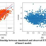Figure 4: (a) Relationship between simulated and observed ETo (b) Residual plot of knnr1 model. Click here to view Figure

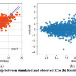Figure 5: (a) Relationship between simulated and observed ETo (b) Residual plot of knnr2 model. Click here to view Figure

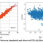Figure 6: (a) Relationship between simulated and observed ETo (b) Residual plot of knnr3 model. Click here to view Figure

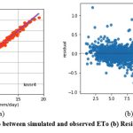Figure 7: (a) Relationship between simulated and observed ETo (b) Residual plot of knnr4 model. Click here to view Figure

Performance of decision tree regression

Similar to knr, the dtr models’ performance with four combinations of meteorological inputs (dtr1, dtr2, dtr3 and dtr4) is discussed in this section.

Determining the ideal leaf sample value is a difficult task. In this study, samples leaf values (2 to 6) are assessed during 5-fold cross validation. The best performance of dtr1, dtr2 and dtr3 models is observed when the samples leaf is configured to 5. Similarly, setting samples leaf to 3 yields the best results from the dtr4 model.

Like knnr1 models, the dtr1 model estimates ETo only with two input parameters (temp._min and temp._max). Table 3 displays the dtr1 model’s performance with 1.04 (SI₁), 1.85 (SI₂), 1.36 (SI₃), 0.91 (SI₄), 0.83 (SI₅). Comparison between observed and predicted ETo by the dtr1 model is shown in Fig. 8(a) with a slope (0.8719) and r² ( 0.8312). The residual description of the dtr1 model is shown in Table 4. Residuals vary from -4.09 to 6.03. The density of residual point can be seen in the range of 2.5-7.5 mm/day on the x axis and -2.0 to 2.0 mm/day on the y axis in Fig. 8(b). Improvement in the predictive skills is noticed in the dtrr2 model, which predicts ETo with temp._min, temp._min, and R_s. Table 3 displays the dtr2 model’s performance with 0.68 (SI₁), 0.91(SI₂), 0.96 (SI₃), 0.96 (SI₄), 0.92 (SI₅). Comparison between observed and predicted ETo by the dtr2 model is shown in Fig. 9(a) with a slope (0.9458) and r² (0.91). The residual description of the dtr2 model is shown in Table 4. Residuals vary from -4.41 to 4.72. The density of residual points can be seen in the range of 2.5-10 mm/day on the x axis and -2.0 to 2.0 mm/day on the y axis in Fig. 9(b). The dtr3 model predicts ETo with temp._min, temp._min, R_s, and u. Table 3 displays the dtr3 model’s performance with 0.47 (SI₁), 0.39 (SI₂), 0.63 (SI₃), 0.98 (SI₄), 0.96 (SI₅). Values of such statistical indicators exhibit that dtr3 shows relatively better performance than the dtr1 and dtr2 models. Comparison between observed  and predicted ETo by the dtr3 model is shown in Fig. 10(a) with a slope (0.9615) and r² (0.96). The residual description of the dtr3 model is shown in Table 4. Residuals vary from -2.80 to 2.29. The density of residual points can be seen in the range of 2.5-12.5 mm/day on the x axis and -1.0 to 1.0 mm/day on the y axis in Fig. 10(b). The best predictive performance is observed in the dtr4 model. It predicts ETo with temp._min, temp._min, R_s u, and R_h. Table 3 displays the dtr4 model’s performance with 0.30 (SI₁), 0.16 (SI₂), 0.40 (SI₃), 0.99 (SI₄), and 0.9856 (SI₅). Comparison between observed and predicted ETo by the dtr4 model is shown in Fig. 11(a) with a slope (0.9709) and r² (0.9856). The residual description in the case of the dtr4 model is shown in Table 4. Residuals vary from -1.92 to 1.44. The density of residual points can be seen in the range of 2.5-10 mm/day on the x axis and -0.5 to  0.5 mm/day on the y axis in Fig. 11(b).

Like knnr models the same interesting finding comes out after analyzing four variants of dtr models (dtr1, dtr2, dtr3, and dtr4) and this indicates that only temperature based models (dtr1) cannot be an appropriate tool to estimate ETo. In addition to temperature, adding solar radiation, wind speed, and humidity makes (dtr4) a more potent and trustworthy tool for estimating ETo.  Another finding reveals that dtr models show less predictive capability than knnr models on all statistical indicators. Similarly, residual plots of dtr3 and dtr4 models are more symmetric about a horizontal line and do not show any specific pattern.

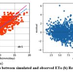Figure 8: (a) Relationship between simulated and observed ETo (b) Residual plot of dtr1 model. Click here to view Figure

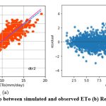Figure 9: (a) Relationship between simulated and observed ETo (b) Residual plot of dtr2 model. Click here to view Figure

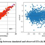Figure 10: (a) Relationship between simulated and observed ETo (b) Residual plot dtr3 model. Click here to view Figure

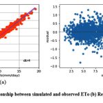Figure 11: (a) Relationship between simulated and observed ETo (b) Residual plot of dtr4 model. Click here to view Figure

Performance of random forest regression

Like knnr and dtr models, the performance of rfr models with four combinations of meteorological inputs (rfr1, rfr2, rfr3 and rfr4) is discussed in this section.

Determining the ideal value of estimators is a difficult undertaking. In this study, estimators values (10 to 100) are assessed during 5-fold cross validation. The best performance of rf1, rfr2 and rfr4 models is observed when the estimators value is set to 100. In the same way, the optimal outcomes for the DTR3 model are obtained when the estimators value is set to 80.

Like kkr1 and dtr1, the rfr1 model estimates ETo only with two input parameters (temp._min and temp._max). Table 3 displays the rfr1 model’s performance with 0.98 (SI₁), 1.7 (SI₂), 1.30 (SI₃), 0.92 (SI₄), (0.84 (SI₅). Comparison between observed and predicted ETo by the rfr1 model is shown in Fig. 12(a) with a slope (0.8658) and r² (0.8438). The residual description of the rfr1 model is shown in Table 4. Residuals vary from -4.26 to 5.46. The density of residual point can be seen in the range of 2.5-7.5 mm/day on the x axis and -2.0 to 2.0 mm/day on the y axis in Fig. 12(b). Similarly, improvement in the predictive skills is noticed in the rfr2 model, which predicts ETo with temp._min, temp._min, and R_s. Table 3 displays the rfr2 model’s performance with 0.611 (SI₁), 0.74 (SI₂), 0.86 (SI₃), 0.97 (SI₄), 0.93 (SI₅). Comparison between observed and predicted ETo by the rfr2 model is shown in Fig. 13(a) with a slope (0.9411) and r2 (0.9324). The residual description of the rfr2 model is shown in Table 4. Residuals vary from -4.26 to 4.16. The density of residual points can be seen in the range of 2.5-10 mm/day on the x axis and -2.0 to  2.0 mm/day on the y axis in Fig. 13(b). The rfr3 model predicts ETo with temp._min, temp._min, R_s, and u. Table 3 displays the rfr3 model’s performance with 0.38 (SI₁), 0.24 (SI₂), 0.49 (SI₃), 0.99 (SI₄), 0.98 (SI₅). Values of such statistical indicators exhibit that rfr3 shows relatively better performance than the rfr1 and rfr2 models. Comparison between observed  and predicted ETo by the rfr3 model is shown in Fig. 14(a) with a slope (0.9569) and r² (0.98). The residual description of the rfr3 model is shown in Table 4. Residuals vary from -2.80 to 2.02 mm/day. The density of residual points can be seen in the range of 2.5 to 12.5 mm/day on the x axis and -1.0 to 1.0mm/day on y the axis in Fig. 14(b). The best predictive performance is observed in the rfr4 model. It predicts ETo with temp._min, temp._min, R_s u, and R_h. Table 3 displays the rfr4 model’s performance with 0.17 (SI₁), 0.049 (SI₂), 0.22 (SI₃), 0.99 (SI₄), and 0.9965 (SI₅). Comparison between observed and predicted ETo by the rfr4 model is shown in Fig. 15(a) with a slope (0.9708) and r² (0.9965). The residual description in the case of the rfr4 model is shown in Table 4. Residuals vary from -1.24 to 0.08. The density of residual points can be seen in the range of 2.5-10 mm/day on the x axis and -0.5 to 0.5 mm/day on the y axis in Fig. 15(b).

Like knnr and dtr models the same interesting finding comes out after analyzing four variants of rfr models (rfr1, rfr2, rfr3, and rfr4) and this indicates that only temperature based models (rfr1) cannot be an appropriate tool to estimate ETo. In addition to temperature, the addition of solar radiation, wind speed, and humidity produces (rfr4) a more potent and trustworthy tool for ETo estimation.  Another finding reveals that knnr and rfr models show similar predictive capability that is better than dtr models. Similarly, residual plots of rfr3 and rfr4 models are more symmetric about a horizontal line and do not show any specific pattern.

As can be seen, combination-4 (temp_min, temp._max, R_s, u, and R_h) exhibits exceptional performance for knnr, rfr, and dtr, with r² values of of 0.99, 0.99 , and 0.98 mm/day, respectively; however, if only a limited amount of meteorological data is taken into account, these models perform poorly. In combination-1, knnr ,rfr and dtr display r2 values of 0.85 , 0.84 0.83 respectively, whereas in combination-2, knnr, rfr and dtr display
r2 values of 0.93, 0.93, 0.91 respectively. Similarly, in combination-3, knnr, rfr and dtr display r2 values of 0.97, 0.97, 0.96 respectively.. It suggests that when variables are increased, models perform better.

Comparison of ETo values calculated by twelve models and FAO_PM56 with the help of box plot is shown in Fig. 16. Box plots of residuals of twelve models are shown in Fig. 17. It can be noticed that knnr4, dtr4 and rfr4 models demonstrate small residuals compared to other models.

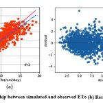Figure 12: (a) Relationship between simulated and observed ETo (b) Residual plot of rfr1 model. Click here to view Figure

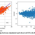Figure 13: (a) Relationship between simulated and observed ETo (b) Residual plot of rfr2 model. Click here to view Figure

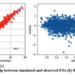Figure 14: (a) Relationship between simulated and observed ETo (b) Residual plot of rfr3 model. Click here to view Figure

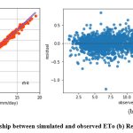Figure 15: (a) Relationship between simulated and observed ETo (b) Residual plot of rfr4 model. Click here to view Figure

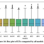Figure 16: Box plot of ETo computed by all models Click here to view Figure

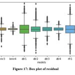Figure 17: Box plot of residual Click here to view Figure

Conclusion

One of the most important services for a country’s economic development is effective water management. It is observed that a huge amounts of freshwater is used in the agriculture sector for irrigation. For the agricultural sector to properly use water, precise and effective methods are needed. Meteorological parameters can play a valuable role in it. Weather stations are outfitted with robust instruments that produce meteorological data in real time. It motivates us to estimate ETo using machine learning algorithms. Models built on machine learning have the capacity to effectively solve challenging non-linear problems and evaluate vast volumes of data. In the present study three regression based machine learning algorithms: k-nearest-neighbors, decision tree  and random forest based models are used to estimate ETo under four categories of input from the weather. Performance is measured on five different statistical indices. The relative findings that come out (1) temperature, solar radiation, wind speed and humidity based models (knnr4, dtr4, and rfr4) demonstrate remarkable performance (r² of 0.9972, 0.9856 and 0.9965 respectively) than those utilizing less meteorological parameters. (2) The knnr and rfr models could be powerful tool than dtr to predict ETo in all combinations of input. (3) Scientists, engineers, and farmers can utilize these knnr and rfr models to schedule irrigation planning, water resource management and crop yield enhancement. In the future, crop water requirements will be estimated by calculating ETc for individual crops using the ETo values derived from these models. 

Acknowledgment

I would like to thanks my P.hD, supervisor, Dr. Anil Kumar Gupta, Head of the Computer Science & Applications Department, Barkatullah University Bhopal(MP) for his guidance and support to carry out this work and complete the article.

Funding Sources

We do not receive any kind of financial support for research and publications.

Conflict of Interest

We do not have any conflict of interest.

Authors’ Contribution

Satendra Kumar Jain: Contributed with the literature review, data collection, model implementation, analysis, and writing the manuscript.

Dr. Anil Kumar Gupta^: Contributed to formulate the problem, design the model, and provide the guidance for writing the manuscript.

Data Availability Statement

Data is taken from India Meteorological Department (IMD) Pune and mentioned in the manuscript.

Ethics Approval Statement 

Not applicable

References

1. Allen RG, Pereira LS, Raes D, Smith M. Crop Evapotranspiration-Guidelines for Computing Crop Water Requirements-FAO Irrigation and Drainage Paper 56.; 1998. Rome, Italy
2. Khosravi K, Daggupati P, Alami MT, et al. Meteorological data mining and hybrid data-intelligence models for reference evaporation simulation: A case study in Iraq. Comput Electron Agric. 2019;167. doi:10.1016/j.compag.2019.105041
   CrossRef
3. Kisi O. Evapotranspiration modelling from climatic data using a neural computing technique. Hydrol Process. 2007;21(14):1925-1934. doi:10.1002/hyp.6403
   CrossRef
4. Gocić M, Motamedi S, Shamshirband S, et al. Soft computing approaches for forecasting reference evapotranspiration. Comput Electron Agric. 2015;113:164-173. doi:10.1016/j.compag.2015.02.010
   CrossRef
5. Feng Y, Cui N, Zhao L, Hu X, Gong D. Comparison of ELM, GANN, WNN and empirical models for estimating reference evapotranspiration in humid region of Southwest China. J Hydrol. 2016;536:376-383. doi:10.1016/j.jhydrol.2016.02.053
   CrossRef
6. Sanikhani H, Kisi O, Maroufpoor E, Yaseen ZM. Temperature-based modeling of reference evapotranspiration using several artificial intelligence models: application of different modeling scenarios. Theor Appl Climatol. 2019;135(1-2):449-462. doi:10.1007/s00704-018-2390-z
   CrossRef
7. Feng Y, Cui N, Gong D, Zhang Q, Zhao L. Evaluation of random forests and generalized regression neural networks for daily reference evapotranspiration modelling. Agric Water Manag. 2017;193:163-173. doi:10.1016/j.agwat.2017.08.003
   CrossRef
8. Fan J, Yue W, Wu L, et al. Evaluation of SVM, ELM and four tree-based ensemble models for predicting daily reference evapotranspiration using limited meteorological data in different climates of China. Agric For Meteorol. 2018;263:225-241. doi:10.1016/j.agrformet.2018.08.019
   CrossRef
9. Yamaç SS, Todorovic M. Estimation of daily potato crop evapotranspiration using three different machine learning algorithms and four scenarios of available meteorological data. Agric Water Manag. 2020;228. doi:10.1016/j.agwat.2019.105875
   CrossRef
10. Tabari H, Martinez C, Ezani A, Hosseinzadeh Talaee P. Applicability of support vector machines and adaptive neurofuzzy inference system for modeling potato crop evapotranspiration. Irrig Sci. 2013;31(4):575-588. doi:10.1007/s00271-012-0332-6
    CrossRef
11. Valipour M, Gholami Sefidkouhi MA, Raeini−Sarjaz M. Selecting the best model to estimate potential evapotranspiration with respect to climate change and magnitudes of extreme events. Agric Water Manag. 2017;180:50-60. doi:10.1016/j.agwat.2016.08.025
    CrossRef
12. Granata F. Evapotranspiration evaluation models based on machine learning algorithms—A comparative study. Agric Water Manag. 2019;217:303-315. doi:10.1016/j.agwat.2019.03.015
    CrossRef
13. Abyaneh HZ, Nia AM, Varkeshi MB, Marofi S, Kisi O. Performance Evaluation of ANN and ANFIS Models for Estimating Garlic Crop Evapotranspiration. J Irrig Drain Eng. 2011;137(5):280-286. doi:10.1061/(asce)ir.1943-4774.0000298
    CrossRef
14. Aghajanloo MB, Sabziparvar AA, Hosseinzadeh Talaee P. Artificial neural network-genetic algorithm for estimation of crop evapotranspiration in a semi-arid region of Iran. Neural Comput Appl. 2013;23(5):1387-1393. doi:10.1007/s00521-012-1087-y
    CrossRef
15. Feng Y, Gong D, Mei X, Cui N. Estimation of maize evapotranspiration using extreme learning machine and generalized regression neural network on the China Loess Plateau. Hydrol Res. 2017;48(4):1156-1168. doi:10.2166/nh.2016.099
    CrossRef
16. Wen X, Si J, He Z, Wu J, Shao H, Yu H. Support-Vector-Machine-Based Models for Modeling Daily Reference Evapotranspiration With Limited Climatic Data in Extreme Arid Regions. Water Resour Manag. 2015;29(9):3195-3209. doi:10.1007/s11269-015-0990-2
    CrossRef
17. Nema MK, Khare D, Chandniha SK. Application of artificial intelligence to estimate the reference evapotranspiration in sub-humid Doon valley. Appl Water Sci. 2017;7(7):3903-3910. doi:10.1007/s13201-017-0543-3
    CrossRef
18. Saggi MK, Jain S. Reference evapotranspiration estimation and modeling of the Punjab Northern India using deep learning. Comput Electron Agric. 2019;156:387-398. doi:10.1016/j.compag.2018.11.031
    CrossRef
19. Mehta R, Pandey V. Reference Evapotranspiration (ETo) and Crop Water Requirement (ETc) of Wheat and Maize in Gujarat. Journal of Agrometeorology. 2015;17(1):107-113. doi: 10.54386/jam.v17i1.984
    CrossRef
20. Wang X, Yao P. A fuzzy KNN algorithm based on weighted chi-square distance. In: ACM International Conference Proceeding Series. Association for Computing Machinery; 2018. doi:10.1145/3207677.3277973
    CrossRef
21. Sutton CD. Classification and Regression Trees, Bagging, and Boosting. Handb Stat. 2005;24:303-329. doi:10.1016/S0169-7161(04)24011-1
    CrossRef
22. Breiman L. Random Forests Machine Learning. 2001;45:5-32. doi:10.1023/A:1010933404324
    CrossRef