Fuzzy Multi-Objective Model for Crop Production Planning with Entropic Disturbance

Introduction

Crop Cultivation is the main sector of INDIA for a major contribution to economic and social development. In agriculture management system plays a significant role in the availability of natural resources in a particular region. Most of the crop production sectors included with favorable agriculture such as compost nature of soil, seasonal factor, labour management, cultivated mix type of crops, maintaining the quantity and quality of crop, fluctuating production etc. can be implemented by successful crop planning and management model. The agriculture production model is usually described as a linear Programming problem. In crop planning and production models, the coefficient of the objective goals/constraints or restrictions parameters are presumed to be a specified certain value. Therefore, there are various diverse circumstances where their exact value remains uncertain that is not be known precisely / accurately and hence uncertainty occurs. So, we need uncertainty-based decision-making methods and here we proposed an uncertainty-based fuzzy programming method. Bellman and Zadeh¹ proposed a fuzzy set theory for decision-making problems in the year 1965. Then 1974 Tanaka et al.² applied Bellman and Zadeh’s concepts of fuzzy set theory. In the crop production planning system, where impreciseness and uncertainty perform a vital role in many judgements of the deterministic situations. Sinha et al.,³ contributes various farm planning problems. Sher and Amir⁴ applied uncertainty-based fuzzy decision-making methods. Nevo et al.⁵ developed an integrated crop planning model for agriculture system. Sarker et al.⁶ formulated a mix crop planning model. Wardlaw and Barnes⁷ described optimum assignment of water supply in cultivation area.

Lodwick et al.⁸ analyses some results by using three different methods for crop production. Itoh and Ishii⁹ studied crop planning problems based on possibility measures. Sarker et al.¹⁰ introduced nationwide crop planning problems using multicriteria decision-making tools. Toyonaga et al.¹¹ introduced a crop production model to obtain reasonable returns with fuzzy random coefficients. An agriculture planning with of goal programming method developed by Biswas and Pal¹² and Sharma et al.¹³ Xieting et al.¹⁴ formulated a mathematical technique for crop production planning. Optimal crop production with several objective was introduced by Rani and Rao.¹⁵ Raluca Andreea et al.¹⁶, and Kumari et al¹⁷ developed different types of crop planning with limited time, resources, budgets etc and reasonably flexible profit at the end of the production. Aminia¹⁸ applied a Fuzzy optimization technique to solve agricultural production model and Sofi et al.¹⁹ Mohamed et al.,^20-21 Sumpsi et al.,²² develop a muti-objective crop production planning problem for the multi farm. Boyabatli et al.,²³ formulated a crop planning in sustainable agriculture and Basumatary and Mitra,^24-25 Mehta and Dwivedi²⁶ described a model of crop planning in a particular area using fuzzy optimization approach. Zandi et al.²⁷ developed an Analytical Hierarchy Process and failure mode and effects analysis–based agricultural risk management framework using fuzzy TOPSIS.

Various optimization methods are used to solve a non-linear problem. The geometric programming (GP)²⁸ is one of the best methods for finding the solution a special type of non-linear optimization models. The dual programming of a GP problem can be described as an entropy optimization of mathematical problem. In 1957 Jaynes’²⁹ introduced an optimization technique called a maximum-entropy principle for finding the distribution of a random system when partial or incomplete data/information is given in the problem Several authors, such as Wilson,³⁰ Kapur,^31-32 Samanta et al.,^33-35 Tsao and Fang,³⁶ Islam and Roy,³⁷ used maximum-entropy principle in various scientific fields mainly Operations Research, engineering and technology etc.

The primary objective of this paper is to optimize crop cultivation within a specific area by employing an entropy objective function as a measure of diversification. This approach facilitates the allocation of farmland across multiple crops and seasons, ensuring responsiveness to market demands while accounting for factors such as profit fluctuations, water availability, skilled labour, and climate uncertainty. The entropy-based model is particularly well-suited for farm managers seeking to diversify crop cultivation in a realistic and sustainable manner.

Formulation of Mathematical Model

A Mathematical Model for Crop Production (MMCP) is considered under the following notations and assumptions:

n = number of different crop cultivation,

m = number of seasons,

c_ij = profit coefficient per unit area for a particular crop i in jth season,           

l_ij = Labour working time for growing crop i in jth season,

b_ij = budget of expenditure per unit area to given Compost, pesticide etc. for crop production for a particular crop i in jth season,

B= Total budget for expenditure,

w_ij = the water requirement for growing crop i in jth season,

z_ij = the required cultivation area for a particular crop i in jth seasons,   

A= gross farm land

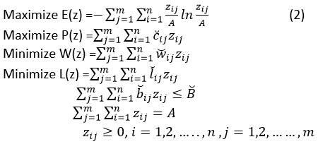
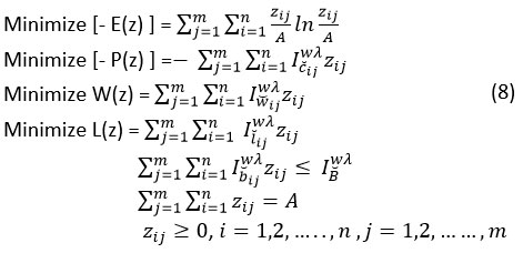
An MMCP model with minimization of Labour time, the requirement of Water Resources and at the same time the maximization of profit objective with maximum entropic disturbance about the partial/incomplete information (i.e. Shannon’s measure of entropy objective function) of farmland distribution under limited farmland and budget for expenditure which can be stated as follows:

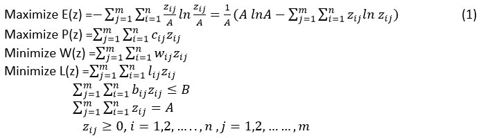
Now MMCP models can be formulated in crisp and fuzzy environments depending upon the nature of the coefficients of objectives, constraints and goals.

Generalized Fuzzy Number and λ-integral Value

The MMCP models are solved with consideration of the coefficient parameters of profits, budget, water availability, labour time etc. given in specific certain data that is crisp environment. But in actual real situations, there are many diversified data caused by uncertainty in decisions, insufficient rain/scarcity of water, changed temperature, pesticide effects, market demand etc. Sometimes it becomes impossible to get applicable specific value. Therefore, this not precise/uncertain value is not at all times well characterized by random variables chosen from a distribution of probability. Hence the different types of data of the MMCP problem may be considered to be not exact/approximated(flexible) i.e. Vague (fuzzy) environment.³⁸

To illustrate, let profit estimation be vaguely expressed and based on subjective management estimation. It may be imprecisely defined as “Profit is about in the range ( P₁, P₂) ” i.e. it may have a value within the left spread interval ( P₁ – δ^—, P₁  ) and right spread interval (P₂, P₂ – δ⁺). Hencethis imprecise profit denoted by quadruplet ( P₁ – δ^–, P₁, P₂, P₂ – δ⁺) may be expressed by the fuzzy set (z, μ_P ̆(z)) with the membership function μ_P ̆(z). The P ̆ represents a trapezoidal fuzzy number P =( P_L, P₁, P₂, P_R) where P_L = P₁ – δ^– and P_R = P₂ – δ⁺ and δ^–, δ⁺, > 0.

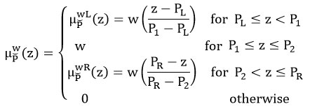
Definition: A fuzzy number P is called Generalized Trapezoidal Fuzzy Number(GTrFN) if P = (P_L, P₁, P₂, P_R, w) where 0 < w ≤ 1 and R_L, P_R are the left and right spread of P₁, P₂ of the range is a fuzzy set in real line R and its membership value (P₁, P₂) is a fuzzy set in real line R and its membership value μ_P^w (z) where μ_P^w (z): R → [0,w] and defined as follows 

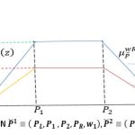Figure 1: Two GTrFN P1 = ( PL, P1, P2, PR , w1), P2 = ( PL, P1, P2, PR , w2) Click here to view Figure

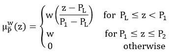
Here the left membership function μ_P^wL (z): [P_L, P₁] → [0,w] is monotonic increasing function and right membership function μ_P^wL (z): [P₂, P_R] → [0,w] is monotonic decreasing function. More generally, the left GTrFN and right GTrFN can be denoted correspondingly by left P = (P_L, P₁, P₂, P₂, w) and right P = (P₁, P₁, P₂, P_R, w) The Left GTrFN P = (P_L, P₁, P₂, P₂, w) provided P_L < P₁  ≤ P₂ (figure 2) is an appropriate word to define concept ‘maximum profit’, ‘larger’, ‘high risk’ etc. in an interval. Therefore, its membership function: 

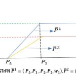Figure 2: Two GTrFN P1 = ( PL, P1, P2, P2 , w1), P2 = ( PL, P1, P2, P2 , w2) Click here to view Figure

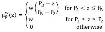
Similarly, the right GTrFN (Figure 3.) of P = (P₁, P₁, P₂, P_R, w) provided P₁ < P₂  ≤ P_R is an appropriate word to define concept ‘minimum cost’, ‘little’, ‘low risk’ etc. in an interval. Therefore, its membership function:

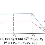Figure 3: Two Right GTrFN P1 = ( P1, P1, P2, PR , w1), P2 = ( P1, P1, P2, PR , w2) Click here to view Figure

Remark 1: If w =1 then the GTrFN is called TrFN.

If P₁ = P₂ then P is called Generalized Triangular Fuzzy Number.

If P₁ = P₂  and w =1 then P is called a Triangular Fuzzy Number.

If P_L = P₁  = P₂  = P₂  = P_R  and w = 1  then P is called  a real number P_R .

Let a pre- assigned parameter λ called the degree of satisfaction / optimism where λ ∈ [0, 1]. The Graded Mean Value(GMV) / Total λ Integral Value (TIV) of P is denoted by I_P^wλ and defined as I_P^wλ = λI_P^wR + (1 – λ) I_P^wL where I_P^wR and I_P^wL represents right and left TIV of  and are defined as 

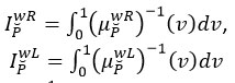
Where (μ_P^wR )^-1 (v) and (μ_P^wL )^-1 (v) represents the inverse of V = μ_P^wR (z) and V = μ_P^wL (z).

If P = (P_L, P₁, P₂, P_R, w) then (μ_P^wR )^-1 (v) = P_R – v-w (P_R – P_Z) and (μ_P^wL )^-1 (v) = P_L – v-w (P₁ – P_L).

Therefore, the right and left integral values are I_P^wR = w-2 (P₂ + P_R) and I_P^wL= w-2 (P_L + P₁). Hence the TIV of P is I_P^wλ = w-2 [λ(P₂ + P_R) + (1 – λ)(P_L + P₁)] The right and left integral values are used to reflect the Optimistic and Pessimistic view points of the decision maker respectively. As one can see TIV is the convex combination of both with optimism degree. Therefore, if λ=1, TIV is I_P^w1 = I_P^wR = w-2 (P₂ + P_R) represents Optimistic viewpoint. When λ=0, TIV is I_P^w0 = I_P^wL = w-2 (P_L + P₁) represents viewpoint of pessimistic situation. Again, if λ=0.5,  the TIV is I_P^w0.5 =  w-4 (P₂ + P_R) + (P_L + P₁) =1-2 (I_P^wR + I_P^wL)  reflects balanced viewpoint or moderately optimistic viewpoint of the decision makers and it turns out to be the same as defuzzification of the fuzzy number P.³⁹

MMCP model with GTrFN

The MMCP model (1) with GTrFN as the coefficients of profit, budget, water availability and labour time of given objective functions which can be represented as follows:

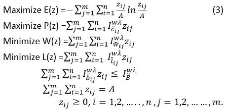
Where c ̆_{ij, b ̆ij, w ̆ij, l ̆ij and B are GTrFN parameters. For left GTrFN}c ̆_ij = (c ̆_ij -c_ij^L, c_ij, c_ij¹, c_ij¹, w ) with the tolerance c_ij^L of the objective function P(z) , the TIV of c_ij, is I_cij^wλ = w-2 [2λc_ij¹ + (1 – λ) (2c_ij – c_ij¹)] Similarly, right GTrFN of w_ij and l ̆_ij are w_ij = (w_ij,w_ij, w_ij¹, w_ij¹ + w_ij^R, w) and l_ij = (l_ij, l_ij, l_ij¹ + l_ij^R, w) with the tolerances w_ij^R and l_ij^R of the objective functions W(z) and L(z) respectively, the TIV are I_wij^wλ = w-2[λ(2w_ij¹ + w_ij^R) + (1 – λ)2w_ij] and I_lij^wλ = w-2[λ(2l_ij¹ + l_ij^R) + (1 – λ)2l_ij]. For right GTrFN of b_ij = (b_ij,b_ij, b_ij¹, b_ij¹ + b_ij^R, w) and B= (B, B, B¹, B¹+ B^R, w) with the tolerances b_ij^R and B^R respectively of ∑_j=1^m  ∑_i=1ⁿ b_ij z_ij ≤ B the TIVs of b_ij and B are I_bij^wλ = w-2[λ(2b_ij¹ + b_ij^R) + (1 – λ)2b_ij] and I_B^wλ = w/2[λ(2B¹ + B^R) + (1 – λ)2B]. Therefore, by using TIV of the fuzzy coefficients, the reformulated form of (2) is

Material and Methods

Fuzzy Nonlinear Programming method

A Set of general m linear or non-linear (or both) objective functions and transform them into the Vector Minimization Form as follows

Subject to z ∈ Z = { z : g_k (z) ≤ d_k, k = 1,2,………,n}

The solution of (4) by using Zimmerman₄₀ Max-Min operator method as following

Where  are corresponding goals of the objective function (z) which are to be minimized and considered these objective functions of (4) as fuzzy constraints. The notation m_r(O_r(z)) represents the membership functions corresponding to O_r(z).  This membership functions are strictly monotonic decreasing function and to calculate payoff table by using Ideal Solution of objective functions and constraints. Hence a set of feasible solution is represented by its membership function is

Now a decision maker can be used a fuzzy optimization method and hence taking maximum level of the feasible solution set, so μ_D (z) 

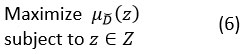
If a ( 0 ≤  a ≤  1 )  be the all compromise satisfactory level then the problem (6)  can be reduced to 

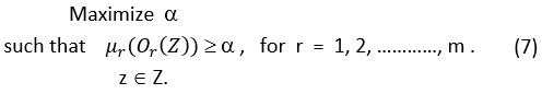
To solve (7) we get Pareto Optimal Solution.

Definition :  Optimal Solution (Complete)

We can said z^* as an optimal solution (Complete) to the problem (4) iff for all z e Z and there exists z^* ϵ  Z such that O_k(z^* )  £ O_k(z),  for k =  1, 2, …, m.

 The Nonlinear problem (4) does not always exist an optimal solution(complete) because many times arises conflict nature of the problems objective functions. Therefore, arises another concept of optimal solution called Optimal Solution (Pareto) as follows:

Definition : Optimal Solution (Pareto)

We can said z^* as an Optimal Solution (Pareto) to the problem (4) iff there does not exist another z ϵ  Z such that for all k =1, 2, ……, m , O_k (z^* )  £ O_k(z) and  for at least one j,  j Π < 1,2,……..,m > , O_j(z ) ¹O_j(z^*).

Solution Procedure of MMCP by using  above solution Procedure

The vector minimization form of problem (3) is

Now to solve the above problem (8), we are used in the above solution procedure. 

Here the membership functions μ_-E[- E(z) ], μ_-P[- P(z) ] , μ_w(W(z)) and μ_L(L(z)) for the objective functions [- E(z)], [- P(z)], W(z) and L(z) respectively are defined as follows:

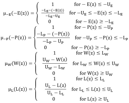
where the U_E , U_P, U_W, U_L and L_E , L_P, L_W, L_L are the upper and lower bounds of the objective functions [- E(z) ], [- P(z) ] ,W(z) and L(z) and its  evaluated by estimated pay off table. 

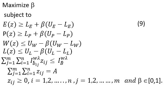
If  β ( 0 ≤ β ≤ 1 )  be the all compromise satisfactory level then the above  problem  (8) is calculated as the following form:

Numerical Example

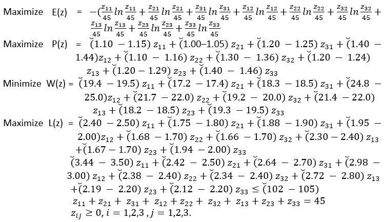
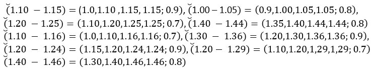
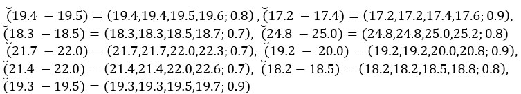
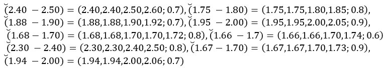
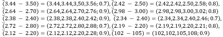
Suppose an agriculture manager assigns their limited farmland areas nearly 45 hectares and he want to grow three types of crops say, Paddy, Brinjal and Red Chili in three different seasons namely Summer, Rainy and Winter. About his past experience, he stated that the total budget of expenditure for cultivation is approximately in the range(interval) Indian Rupees 102 lakhs to 105 lakhs, The following table represents the range of budget for expenditure ( in lakhs), work time( in day=24 hours) for labour and water availability( in hector-inches)  for the crop production per unit hector area and his past three year ( three seasons) experience of profit coefficients range ( in lakh) to grow five different crop  are given:

Table 1: Season wise Crop information

Season (j)	Crop Name (i)	Profit coefficients ( lakhs)	Water availability (hector-inches)	Work time for Labour (days)	Budget for expenditure (lakhs)
Summer Season	Paddy (z11)	1.10 –1.15	19.4 –19.5	2.40 –2.50	3.44 – 3.50
	Brinjal(z21)	1.00 – 1.05	17.2 –17.4	1.75 –1.80	2.42 – 2.50
	Red Chili(z31)	1.20 –1.25	18.3 –18.5	1.88 –1.90	2.64 – 2.70
Rainy Season	Paddy (z12)	1.40 –1.44	24.8 –25.0	1.95 –2.00	2.98 – 3.00
	Brinjal(z22)	1.10 – 1.16	21.7 –22.0	1.68 –1.70	2.38 – 2.40
	Red Chili(z32)	1.30 – 1.36	19.2 – 20.0	1.66 –1.70	2.34 – 2.40
Winter Season	Paddy (z13)	1.20 – 1.24	21.4 –22.0	2.30 –2.40	2.72 – 2.80
	Brinjal(z23)	1.20 – 1.29	18.2 –18.5	1.67 –1.70	2.19 – 2.20
	Red Chili(z33)	1.40 – 1.46	19.3 –19.5	1.94 –2.00	2.12 – 2.20

The Manager assigned his farmland areas i.e.  cultivation land area of the corp i ( i=1,2,3,4.5 ) in  jth ( j=1,2,3) season, therefore the mathematical formulation of imprecise  / flexible  data of different coefficients and goals , so the model are as follows:          

 Where fuzzy objective coefficient of P(z) is

Similarly fuzzy objective coefficient of W(z) is

 and fuzzy objective coefficient of L(z) is

Fuzzy Coefficients and goals of Budget constraints is

Results

For any value of l in [0, 1], say l =0.50 then the pareto Optimal solutions are as follows (table-2):

Table 2: Optimal solutions (Pareto) of MMCP Model for λ =0.50

Variables and Objective Function	MMCP Model (without Entropy)	MMCP Model (with Entropy)
Z*11	0.000000	1.285761
Z*21	0.000000	0.7854402
Z*31	19.20409	15.51402
Z*12	0.000000	0.09550524
Z*22	0.000000	1.129301
Z*32	23.33358	19.00942
Z*13	2.462324	1.871013
Z*23	0.000000	1.855958
Z*33	0.000000	3.453579
P(Z*)	46.14557	45.68658
W(Z*)	701.4866	707.1461
L(Z*)	53.81290	56.08869
E(Z*)	———–	1.469690

Table-3: Optimal solutions(Pareto) of MMCP Model for different λ

Test	β*	E(Z*)	P(Z*)	W(Z*)	L(Z*)
Optimistic i.e. l λ =1.0	0.5171632	1.466057	47.67087	720.8760	57.16139
About Optimistic i.e. l λ = 0.80	0.5175277	1.468059	46.88355	715.3293	56.72653
Moderate i.e. l λ = 0.50	0.5174324	1.469690	45.68658	707.1461	56.08869
Pessimistic i.e. l λ =0.0	0.5119525	1.463074	45.60090	694.3912	55.13732

Discussion

The above table (Table 2) shows that the MMCP model without the entropy objective has most variables (z₁₁^*, z₂₁^*, z₁₂^*, z₂₂^*, z₂₃^*, z₃₃^*​) equal to zero, whereas in the MMCP model with the entropy objective function, all variables take non-zero values. In this problem, the entropy objective function serves as a measure of diversification, disorder, or dispersal in farmland allocation, encouraging cultivation of all crop types across different seasons to meet market demand, even with only minor changes in the objectives (profit (P(z*)), water availability (W(z*)) and labour time (L(z*))). For a farmer aiming to distribute farmland across different crop types, the MMCP model with an entropy objective function offers a more realistic solution. Hence, the entropy-based model is more applicable in real scenarios, as it balances maximum profit and minimal water and labour requirements (with only very small changes) while ensuring maximum entropy in farmland distribution.

Conclusion

This study presents various types of crop cultivation for agricultural management systems in different seasons. Here, the given article is to formulate the mathematical model for a crop production problem in a fuzzy environment with diversification (Entropy optimization) as an Entropy Maximization problem. Therefore, this entropy objective function acts as a measure of diversification/disorder/dispersal of farmland distribution to cultivate all types of crops in different seasons due to need of market demands with very small changes of objective values of profit, water availability and human resource (labour time). A nonlinear fuzzy decision-making method is employed to solve this real-life problem, specifically farm management for cultivating different crops. Like crop production planning and management problems, this method (Entropy optimization with fuzzy environments) can be applied to the problems of other fields such as Polyculture, Risk Analysis, Engineering Optimization, Environmental Analysis, etc.

Acknowledgment

The author gratefully acknowledges the faculty members of the Department of Mathematics, Hijli College, for their support and encouragement throughout this research work.

Funding Sources

The author(s) received no financial support for the research, authorship, and/or publication of this article.

Conflicts of Interest

The authors do not have any conflict of interest.

Data Availability Statement

This statement does not apply to this article.

Ethics Statement

This research did not involve human participants, animal subjects, or any material that requires ethical approval.

Informed Consent Statement

This study did not involve human participants, and therefore, informed consent was not required.

Permission to Reproduce Material from other Sources

Not Applicable.

Author Contributions

The sole author was responsible for the conceptualization, methodology, data collection, analysis, writing, and final approval of the manuscript.

References

1. Bellman, R. E., Zadeh, L. A. Decision-making in a fuzzy environment, Management Sciences;1970;17 (4): 141-164.
   CrossRef
2. Tanaka H., Okuda T., Asai K. On fuzzy mathematical programming, Journal of Cybernetics;1974;3(4): 37-46.
   CrossRef
3. Sinha S. B., Rao K.A., Mangaraj B.K. Fuzzy goal programming in multicriteria decision systems –A Case study in agriculture planning, Socio-Economic Planning Sciences;1988; 22(2):93-101. https://doi.org/10.1016/0038-0121(88)90021-3
   CrossRef
4. Sher, Amir I. Optimization with fuzzy constraints in Agriculture production planning, Agricultural Systems;1994; 45:421-441. DOI:10.1016/0308-521X(94)90133-Z
   CrossRef
5. Nevo, A., Oad, R., Podmore, T.H. An integrated expert system for optimal crop planning. Agricultural Systems;1994; 45(1): 73-92. https://doi.org/10.1016/S0308-521X(94)90281-X
   CrossRef
6. Sarker R. A., Talukdar S., Anwarul Haque A.F. M. Determination of optimum crop mix for crop cultivation in Bangladesh, Applied Mathematical Modeling;1997;21 : 621-632.
   CrossRef
7. Wardlaw, R., Barnes, J. Optimal allocation of irrigation water supplies in real time, Journal of Irrigation and Drainage Engineering;1999;125:345–354
   CrossRef
8. Lodwick W., Jamison D., Russell S. A comparison of fuzzy stochastic and deterministic methods in Linear Programming, Proceeding of IEEE; 2000: 321-325.
   CrossRef
9. Itoh T., Ishii H., Nanseki T. A model of crop planning under uncertainty in agriculture management, J. Production Economics; 2003; 81-82: 555-558. DOI:10.1016/S0925-5273(02)00283-9
   CrossRef
10. Sarker, R.A., Quaddus, M.A. Modelling a nationwide crop planning problem using a multiple criteria decision making tool, Computers & Industrial Engineering;2002;42(2-4): 541-553. https://doi.org/10.1016/S0360-8352(02)00022-0
    CrossRef
11. Toyonaga T., Itoh T., Ishii H. A crop planning problem with fuzzy random profit coefficients, Fuzzy Optimization and decision making;2005; 4,: 51-59. DOI:10.1007/s10700-004-5570-5
    CrossRef
12. Biswas, B., Pal, B. Application of fuzzy goal programming technique to land use planning in agriculture system, Omega;2005; 33: 391-398. DOI:10.1016/j.omega.2004.07.003
    CrossRef
13. Sharma, D. K., Jana, R.K. Fuzzy goal programming for agricultural land allocation problems, Yugoslav Journal of Operation Research;2007;17(1) :31-42.
    CrossRef
14. Xieting, Z., Shaozhong, K., Fusheng, L. Lu, Z. Ping, G. Fuzzy Multi-Objective linear programming applying to crop area planning, Agricultural Water management;2010;98(1):134-142.
    CrossRef
15. Rani, Y.R., Rao, D.P.T. Multi objective crop planning for optimal benefits, International Journal of Engineering Research;2012; 2(5): 10.
16. RalucaAndreea, I., TurekRahoveanu, A. Linear Programming in Agriculture: Case Study in Region of Development South-Mountenia, International Journal of Sustainable Economies Management; 2012; 1: 51-60. doi=10.4018/ijsem.2012010105
    CrossRef
17. Kumari P.L., Reddy G.K., Krishna T.G. Optimum Allocation of Agricultural Land to the Vegetable Crops under Uncertain Profits using Fuzzy Multiobjective Linear Programming , Journal of Agriculture and Veterinary Science; 2014; 7(12) : 19-28 DOI:10.9790/2380-071211928
    CrossRef
18. Aminia, A. Application of Fuzzy Multi-Objective programming in Optimization of crop production planning, Asian Journal of Agricultural Research; 2015;9(5): 208-222.
    CrossRef
19. Sofi, N.A., Ahmed, A., Ahmad, M., Bhat, B.A. Decision making in agriculture: A linear programming approach, Economics;2015;13(2): 160-169.
20. Mohamad, N., Said, F. A mathematical programming approach to crop mix problem; African Journal of Agricultural Research;2011;6(1):191-197. DOI: 10.5897/AJAR10.028
21. Mohamed, H.I., Mahmoud, M.A., Elramlawi, H.R.K., Ahmed, S.B. Development of mathematical model for optimal planning area allocation of multi crop farm, International Journal of Science and Engineering Investigations;2016; 5(59): 7.
22. Sumpsi J. M., Francisco A., Carlos, R. On Farmer‟s Objectives: A multi criteria approach, European Journal of Operation Research;1996; 96:64-71.
    CrossRef
23. Boyabatlı, O., Nasiry, J., Zhou, Y. Crop planning in sustainable agriculture: dynamic farmland allocation in the presence of crop rotation benefits, Management Science;2019; 65(5): 1949-2443. https://doi.org/10.1287/mnsc.2018.3044
    CrossRef
24. Basumatary, U.R., Mitra, D.K. A Study on optimal land allocation through Fuzzy Multi-Objective Linear Programming for Agriculture production planning in Kokrajhar District, BTAD, Assam, INDIA, International Journal of Applied Engineering Research;2020;15(1) : 94-100.
25. Basumatary, U. R., Mitra, D. K. Different size group of farmers crop production planning using multi-objective fuzzy linear programming in chirang district btad, assam, india, Advances in Mathematics: Scientific Journal; 2020; 9(10): 8077–8089, https://doi.org/10.37418/amsj.9.10.40
    CrossRef
26. Mehta, S., Dwivedi, R.K. Crop planning using Fuzzy Optimization Technique-A case study of Hazaribag district, Jharkhand, Journal of Emerging Technologies and Innovative Research;2019;6(4):344-349.https://www.jetir.org/papers/JETIR1904T48.pdf
27. Zandi, P., Rahmani, M., Khanjan, M., Mosavi, A. Agricultural Risk Management Using Fuzzy TOPSIS Analytical Hierarchy Process (AHP) and Failure Mode and Effects Analysis (FMEA), Agriculture, 2020;10(504):1-27.https://doi.org/10.3390/agriculture10110504
    CrossRef
28. Duffin, R.J. , Peterson, E.L. and Zener, C., Geometric Programming—Theory and Application, Wiley, New York, 1967.
29. Jaynes, E. T. Information theory and statistical mechanics, The Physical Review; 1957 ;108 : 171-190.
    CrossRef
30. Wilson, A.G. Entropy in Urban and Regional Modelling, Pion, London, 1970.
31. Kapur J. N., Maximum-Entropy Models in Science and Engineering, Revised ed, Wiley Eastern Limited, New Delhi, 1993.
32. Kapur J. N.and Kesavan H. K., Entropy Optimization Principles with Applications, Academic Press, Inc., San Diego, 1992.
    CrossRef
33. Samanta B., Majumder S.K. Entropy based Transportation model use Geometric Programming method, Journal of Applied mathematics and Computation;2006;179: 431-439 DOI:10.1016/j.amc.2005.11.154
    CrossRef
34. Samanta, B. Entropy based multi-objective Matrix game model with Fuzzy goals, Tamsui Oxford journal of Information and Mathematical Science;2017;31(2):82-92.
35. Samanta, B. Fuzzy Multi objective Matrix Game: An Entropic Uniformity Approach, Science and Technology Journal;2020;8(1):52-57.
    CrossRef
    
36. Tsao H. S. J., Fang S. C. Linear Programming with inequality constraints Via entropic perturbation, J. of math. and math. Sci.;1996; 19(1):177-184.
    CrossRef
37. Islam, S., Roy,T.K. A new fuzzy multi-objective programming: Entropy based geometric programming and its application of transportation problems, European Journal of Operational Research; 2006; 173 : 387–404
    CrossRef
38. Zadeh, L. A.  Fuzzy sets, Information and Control;1965; 8:338-353.
    CrossRef
39. Kaufmann, A., Gupta M. M. Fuzzy mathematical models in engineering and management science, North-Holland ,1988.
40. Zimmermann, H.J. Fuzzy programming and linear programming with several objective functions, Fuzzy Sets and Systems;1978; 1: 45-55.
    CrossRef